
Have you ever created a chart in Google Sheets with multiple series, and you wanted to change the order of the series? Before I learned how to do this I would always change the order of the data, instead of simply changing the order of the series on the chart itself.
In this lesson I am going to show you multiple ways to easily change the series order on charts in Google Sheets.
To change the series order on a chart in Google Sheets, double-click no the chart to open the chart editor, scroll down to the “Series” section on the “Setup” tab, click the three dots on a series and then click “Remove” to remove any series that is not in the correct order, and then click “Add series” to add the series again in the order that you wish.
Below is a detailed example with example images.
Click here to learn how to create / customize charts in general.
Change the series order on a chart (in the chart editor)
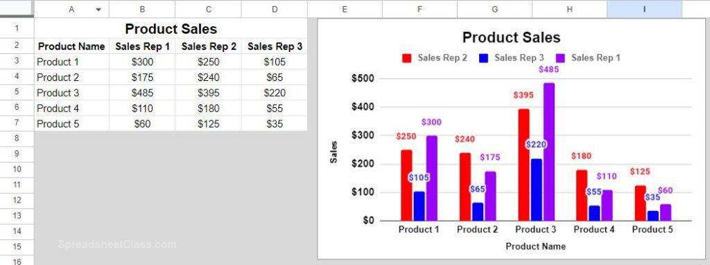
In this example, we are going to change the series order on a column chart. The column chart below displays how much money that three different sales representatives made on a variety of products. There are 3 sales reps, and each one is a series on the chart.
As you can see in the image below, the chart has the series listed in the wrong order, where sales rep 2 is the first series, sales rep 3 is the second series, and sales rep 1 is the third series.
We are going to change the series order so that sales rep 1 is the first series, where sales rep 2 is the second series, and where sales rep 3 is the third series.
To do this we are going to remove the series for sales rep 2 and sales rep 3 (which will leave sales rep 1 as the first / only series), and then we will add the series other sales reps / series back again, in the correct order (sales rep 2, then sales rep 3).
To change the series order for the chart, follow the steps below.
Click here to get your Google Sheets cheat sheet
Or click here to take the dashboards course
Double-click on the chart to open the chart editor (Another way to open the chart editor, is to click once on the chart, then click the 3 dots in the upper-right corner, and then click “Edit chart”)
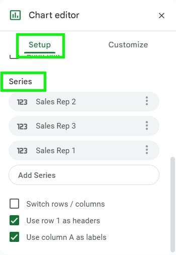
On the “Setup” tab, scroll down to the section that says “Series”
You will see the order that the series on the chart are in here. The series on top will display first on the chart / legend, and the series on bottom will display last on the chart)
As you can see, the sales reps are in the following order (2, 3, 1). We want to change the order to (1, 2, 3). To do this we want to start by making sure that the first sales rep is the first series. We will need to remove any series that is in a higher position than it should be. In this case we must remove the first and second series to assure that sales rep 1 is in the first position / is the first series.
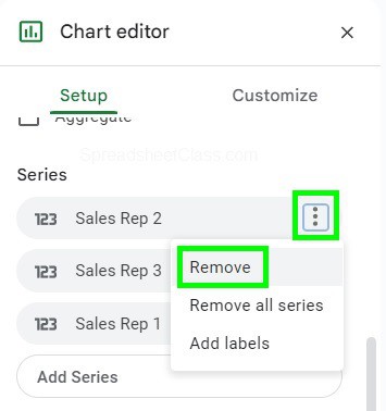
Click the 3 dots on each series to be remove, and then click “Remove”
After removing sales rep 2 and sales rep 3… sales rep 1 is the only series on the chart, and is in the first position / is the first series like we want. Now you can add the other series in the correct order.
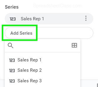
Click “Add series”, then click the next series that you want to add, in this case we will add “Sales rep 2”. Repeat the process for sales rep 3.
As you can see in the image below, both the chart editor and the chart itself now show the sales reps / series in the correct order (1 2, 3).
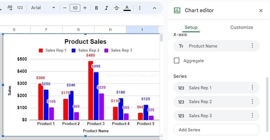
Note that we were able to change the series order on a chart in Google Sheets without having to change the order of the columns in the raw data!
Changing series order vs. changing order of columns in the data
Before I discovered how to change the series order directly on a Google Sheets chart, I used to change the order of the columns in the data that the chart was connected to.
This is also an option if you want… but if you click and drag (or cut and paste) the columns to change the order of the columns, it may automatically remove one or more of the series from the chart when you do this, and it may also modify the data range that the chart is connected to. In this case you would need to open the chart editor, assure that the data range is correctly set, and remove / add the series as needed.
If you switch the column order by pasting or entering new values to swap the data in each column (without moving or cutting the column itself), then this will change the order of the series on the chart without having to open the chart editor.
A great way to do this is by copying and pasting values only, by using Ctrl +C to copy, and then pressing Ctrl + Shift + V to paste values only.
More examples of changing series order
Let’s go over some more scenarios / steps for changing the series order in Google Sheets, so that you can get a full understanding of how to reorder the chart series put them in the exact order that you want.
In each example, first you will see the initial order that the series are in. Then you will see the order that we want to put the series in. Then you will see the steps to take in each case, to change the order as desired.
Example 1
Series order:
Jacob, Bill, Barry, Thomas
Desired order:
Jacob, Bill, Thomas, Barry
Steps to reorder series:
Remove Barry, add Barry
Example 2
Series order:
Friday, Wednesday, Monday, Thursday, Tuesday
Desired order:
Monday, Tuesday, Wednesday, Thursday, Friday
Steps to reorder series:
Remove Friday, remove Wednesday, remove, Thursday, add Wednesday, add Thursday, add Friday
Now you know multiple ways to change the series order on a chart in Google Sheets!
This content was originally created by Corey Bustos / SpreadsheetClass.com

