
In Google Sheets it’s common to need to alphabetize your data, and there are multiple easy ways to do it. In this article I will show you how to alphabetize your lists and your data, by manually sorting without a formula, and I will also show you how to alphabetize your data by using the SORT function. I’ll teach you how to sort data in ascending (A to Z) or descending (Z to A) order.
To alphabetize in Google Sheets, select the range that you want to alphabetize, click “Data”, and then click “Sort sheet (A to Z)”.
Alternatively, you can right-click on the column that you want to sort, and then click “Sort sheet A to Z”
Method 1: Alphabetize Without a Formula (Manual Sorting)
First let’s go over how to alphabetize manually, by using the menu option.
To alphabetize in ascending order, follow these steps:
- Select the Range of cells that you want to alphabetize
- Click the “Data” menu on the top toolbar
- Hover your cursor over “Sort sheet”
- Click “Sort sheet (A to Z)”
After following the steps above, Google Sheets will automatically reorder the rows in ascending order, based on the selected column.
To alphabetize in descending order, follow these steps:
- Select the Range of cells that you want to alphabetize
- Click the “Data” menu on the top toolbar
- Hover your cursor over “Sort sheet”
- Click “Sort sheet (Z to A)”
After following the steps above, Google Sheets will automatically reorder the rows in descending order, based on the selected column.
How to alphabetize in Google Sheets
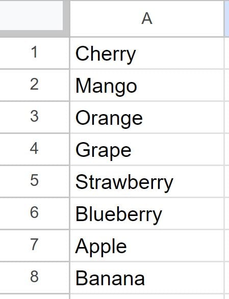
Let’s say that you have a list of fruits in column A and you want to alphabetize them.
The image below shows the unsorted list of fruits.
Alphabetize in ascending order
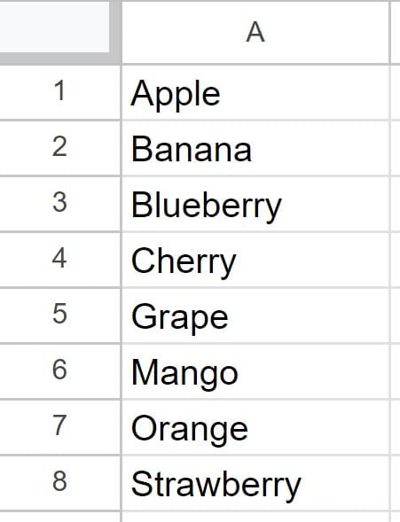
In this example we will sort the list of fruits in ascending order. To do this follow the steps below.
- Select column A
- Click “Data” on the top toolbar menu.
- Hover your cursor over “Sort sheet”
- Click “Sort sheet by Column A (A to Z)”

After following the steps above, the data will be alphabetized, as shown in the image below.
Alphabetize in descending order
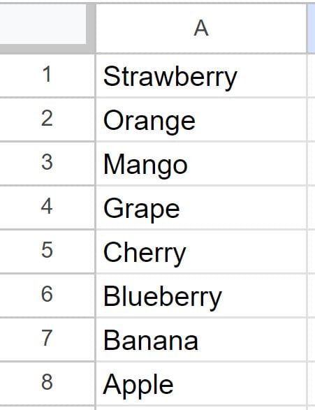
In this example we will sort the list of fruits in descending order. To do this follow the steps below.
- Select column A
- Click “Data” on the top toolbar menu.
- Hover your cursor over “Sort sheet”
- Click “Sort sheet by Column A (Z to A)”

After following the steps above, the data will be sorted in descending order, as shown in the image below.
Method 2: Alphabetize With a Formula (SORT Function)
Now let’s go over how to alphabetize by using the SORT function, which will automatically alphabetize your data after the formula is entered. Click the article above to learn more detail about using the SORT function.
The SORT function sorts a specified range, by a specified column, in a specified order. For the sort order, enter TRUE to sort in ascending order, or enter FALSE to sort in descending order. The examples below demonstrate this.
Sort in ascending order with the SORT function:
In this example, we will sort a list of countries in ascending order by using the SORT function.
=SORT(A1:A, 1, TRUE)
The formula above (entered into cell B2) sorts the data in column A (A1:A) in ascending order (TRUE).
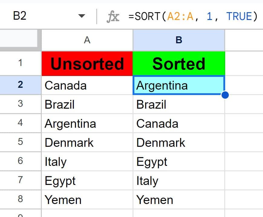
As you can see in the image above, the SORT function generated a sorted list of countries, in ascending order.
Sort in descending order with the SORT function:
In this example, we will sort a list of countries in descending order by using the SORT function.
=SORT(A1:A, 1, FALSE)
The formula above (entered into cell B2) sorts the data in column A (A1:A) in descending order (FALSE).
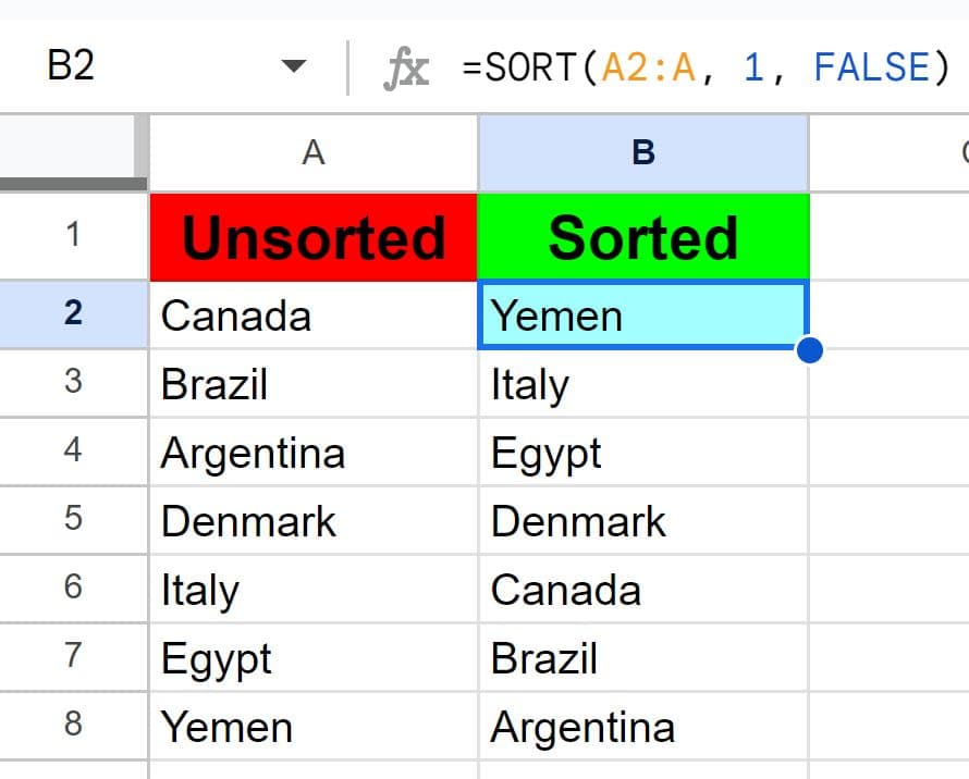
As you can see in the image above, the SORT function generated a sorted list of countries, in descending order.
Now you know all the ways to alphabetize in Google Sheets!

