
Checkboxes are a very handy and versatile tool to use in Google spreadsheets, and so in this article I am going to show you how to insert checkboxes into your Google Spreadsheet. I’ll also show you several ways to use checkboxes, how to format them, how to remove them, and more.
To insert a checkbox in Google Sheets, click on the cell that you want to add a checkbox to, click “Insert” on the top toolbar, then click “Checkbox”. If you want to add checkboxes to multiple cells, select multiple cells, and then click “Insert”, then click “Checkbox” and Google Sheets will add checkboxes to each cell that was selected.
Simply click on a checkbox once to check the box, and click on it again to uncheck the box. If you need to select a cell that contains a checkbox without checking / unchecking the checkbox, simply click inside of the cell, but outside of the checkbox.
You can also copy and paste checkboxes to duplicate them while keeping any formatting. Below I’ll tell you how to do this, and I’ll teach you all that you need to know about checkboxes.
Check out the to-do list / checklist template for Google Sheets
Get your Google Sheets formulas cheat sheet
How checkboxes work (True vs. False, Checked vs. Unchecked)
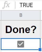
A checkbox is like an on / off switch, it is either checked (TRUE) or unchecked (FALSE). Even though the checkbox will display in the spreadsheet cell, you will see that when you select a cell with a checkbox in it, the formula bar on the top of the spreadsheet will display the text “TRUE” if the checkbox is checked, or it will display the text “FALSE” if the checkbox is unchecked.
This is important because this TRUE / FALSE state will allow us to interact with checkboxes by using formulas, such as sorting a list by checkbox status or filtering a list where only the unchecked boxes are displayed. I will show you how to use formulas with checkboxes later.
Note in the image directly below, the checkbox is checked, and since the cell that contains the checkbox is selected, the formula bar says “TRUE”.
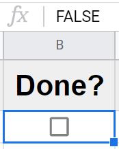
Note in the image directly below, the checkbox is unchecked, and since the cell that contains the checkbox is selected, the formula bar says “FALSE”.
Inserting a checkbox in Google Sheets (Example)
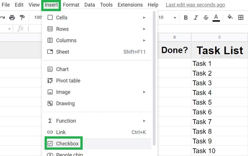
So now let’s go over a basic example of inserting a checkbox in Google Sheets. As you can see in the image below, we have a list of tasks in column C, and we want to start by inserting a checkbox at the top of column B, to use as an indication of whether the task has been completed or not.
To insert a checkbox into your spreadsheet, follow the steps below.
Select the cell that you want to add a checkbox to (cell B2 in this case)
On the top toolbar, click “Insert”
Click “Checkbox”
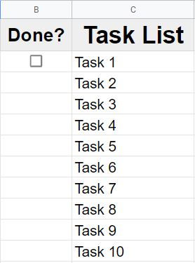
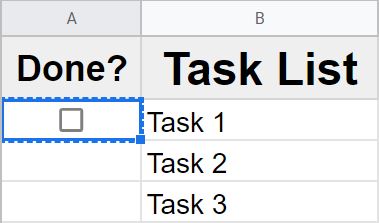
As you can see in the image below, after following the steps above, a checkbox has now appeared in cell B2.
Copying and removing checkboxes in Google Sheets
You can easily duplicate checkboxes by copying and pasting the cells that contain a checkbox. For example, after inserting the checkbox from the previous example, let’s say that we want to copy the checkboxes down the column. This can be done by copying and pasting or using the fill handle.
Removing checkboxes
Removing checkboxes is very easy, simply select the cell(s) that you want to remove a checkbox from, and then press “Backspace” or “Delete” on the keyboard.
This will completely remove the checkboxes from the cells.
Copying and pasting checkboxes
Top copy and paste checkboxes, select the cell that contains the checkbox that you want to duplicate, press Ctrl + C on the keyboard to copy the cell, select the cell where you want to copy the checkbox to, then press Ctrl + V to paste. The cell that you paste into will now have a checkbox as well.
Repeat this until all the cells that you want have checkboxes. If you select a range of cells before pasting, the entire range will be filled with checkboxes.
Using the fill handle to copy checkboxes
You can also use autofill / the fill handle to copy checkboxes.
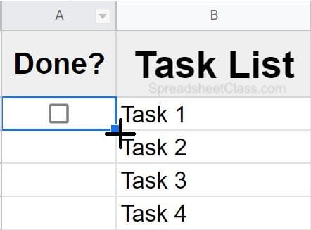
To copy checkboxes with autofill, select the cell that contains the checkbox that you want to copy, hover your cursor over the bottom-right of the cell until a plus sign / crosshairs appears, click your mouse, hold the click, then drag your cursor downwards until you reach the cell where you want to copy the checkboxes to, then release your click.
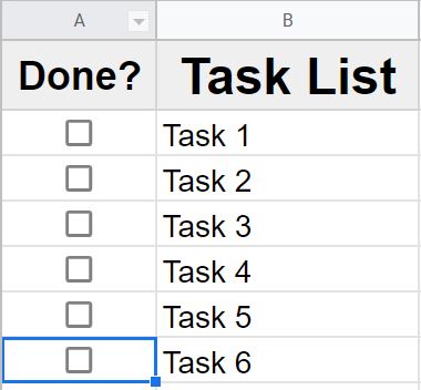
The image directly below shows what the sheet looks like after copying the checkboxes down the column.
Formatting checkboxes (Color & Size) in Google Sheets
Checkboxes can be formatted in several ways, and it’s very easy to do.
The font size of the cell will control the size of the checkbox.
The text color of the cell will control the color of the checkbox.
The fill color of the cell will control the background color of the checkbox.
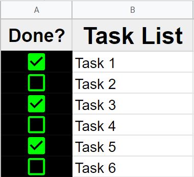
As you can see in the image below, the font size is set to green, the fill color is set to black, and the font size has been increased from the default. So the checkboxes are bigger, the checkboxes are green, and the background color for the checkbox is black.
How to sort by checkboxes in Google Sheets
In this example we are going to sort a list / sheet, and we are going to sort by the status of the checkboxes in column A. In the next example I’ll show you how to do this by using a formula, but in this example we will sort by using the menu option in Google Sheets.
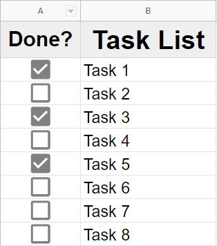
As you can see in the image below, some of the tasks have a checked checkbox beside them, and some of them have unchecked checkboxes beside them. We are going to sort the data so that the rows with unchecked checkboxes rise to the top, and the rows with checked checkboxes will go to the bottom (leaving incomplete tasks at the top as we want).
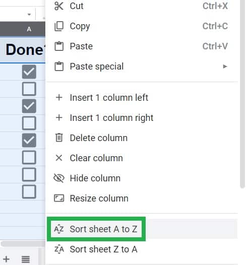
To sort by checkboxes in Google Sheets, right-click on the column with the checkboxes in it, and then click “Sort sheet A to Z” (or to sort in reverse order you can choose “Sort sheet Z to A”
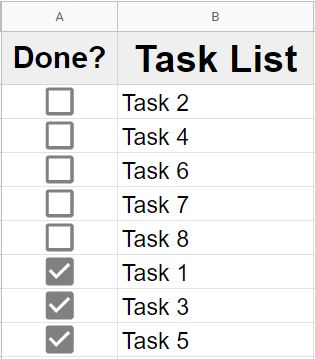
When you choose “Sort sheet A to Z”, the unchecked checkboxes (FALSE state) will rise to the top of the sorted list, as shown in the image below.
Now all of the incomplete tasks are grouped together at the top of the list, exactly how we wanted.
How to sort with a formula in Google Sheets
Now let’s go over an example of sorting checkboxes, but this time we will sort by using a formula. Note that when we sort data by checkboxes with a formula, the results will display text designating the TRUE / FALSE state of the checkboxes, rather than showing the checkboxes themselves.
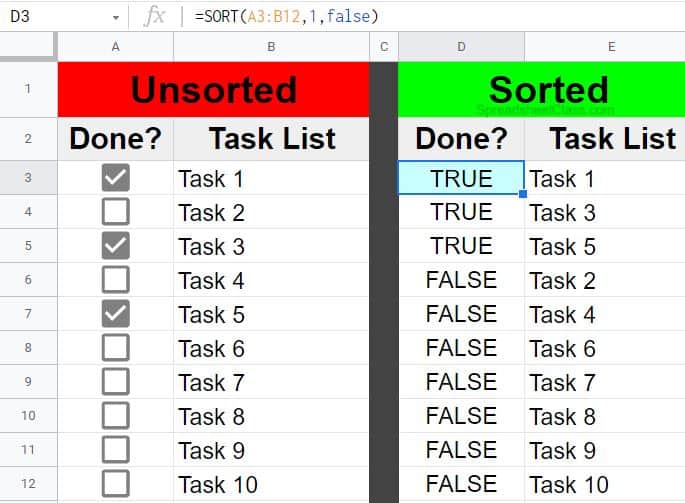
To use the SORT function, type an equals sign (=), then type the range that you want to sort (such as “A3:B12”), type a comma and then enter the number of the column to sort by (such as “1”), type a comma and then type “false” to sort in descending order (or “true” for ascending order). Your final formula will look like this: =SORT(A3:B12,1,false)
So in this example we are sorting columns A and B, by column 1 (contains the checkboxes), and we are sorting in descending order.
As you can see in the image below, after entering the formula above in cell D3, the list of tasks has now been sorted according to the status of the status of each checkbox in column A. Now the complete tasks are at the top of the sorted list (TRUE / checked checkboxes), and the incomplete tasks are at the bottom of the sorted list (FALSE / unchecked checkboxes).
Create a custom checkbox with data validation
If you want, you can use “Data validation” to create a checkbox, and with this method you can customize the checkbox, such as being able to choose which values you want to assign to the checked / unchecked state of the checkbox (default is TRUE / FALSE). So you can make it so the checkboxes display Yes / No, instead of True / False, if you want… or you can choose any custom value to assign that you want.
You can also choose to show a warning or reject input if someone enters anything into the cell other than the set values for the checkbox.
To add a checkbox by using data validation, follow these steps:
- Select the cell(s) that you want to add a checkbox to
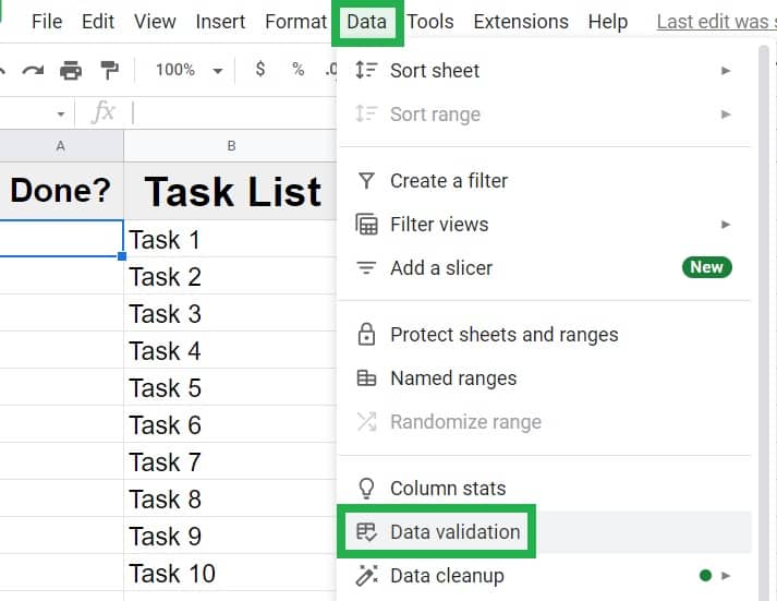
- Click “Data” on the top toolbar
- Click “Data validation”
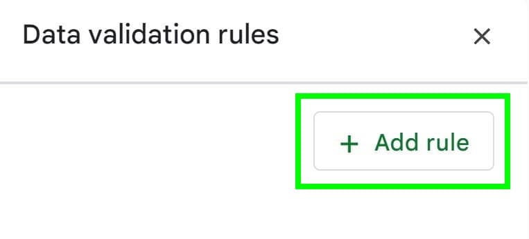
- Click “Add rule”
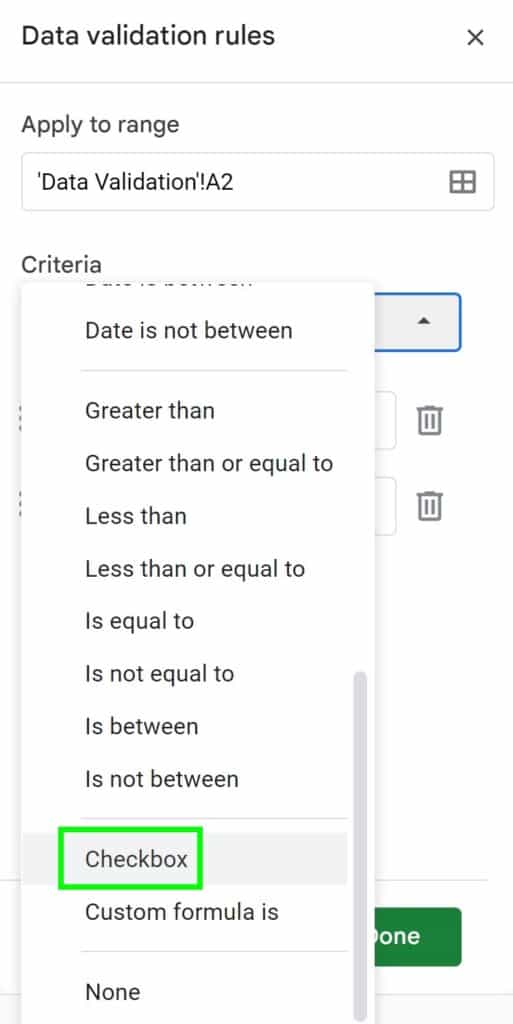
- Click the “Criteria” dropdown
- Scroll down and click “Checkbox”
Here are the steps for adding a checkbox with data validation, with example images included.
Click “Data”, and a menu will pop up. Click “Data validation” and a menu will appear on the right.
Click “Add rule”
Click on the dropdown menu that says “Criteria”, then scroll down and click “Checkbox”
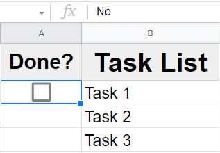
After following the steps above, a checkbox will appear in the cell, as shown in the image below.
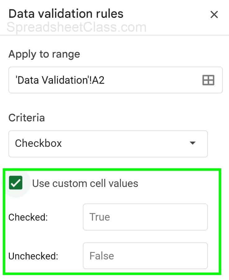
Customizing checkbox values
You can set custom values for the checkbox to designate which text that you want to be associated with the check / unchecked state for the checkbox (default is TRUE / FALSE).
To set custom values for the checkbox, follow these steps:
- Select the cell(s) that contain the checkboxes that you want to choose custom values for
- Click “Data” on the top toolbar
- Click “Data validation”
- Select the “Checkbox” rule
- Click the checkbox that says “Use custom cell values”
- Enter the values that you want to associate with the Checked / Unchecked states (Such as “Yes and “No”, or “Complete” and “Incomplete”)
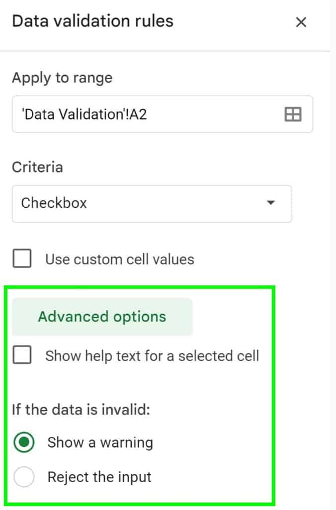
Choosing to show a warning vs. reject the input for checkboxes
While editing a checkbox data validation rule, you can also choose whether the cell will “Show a warning” if someone enters a value other than the specified (or default) checkbox values… or you can choose “Reject the input”.
With “Show a warning” selected (default), when someone enters text into the cell other than “TRUE” or “FALSE”, Google Sheets will show a warning. This warning displays as a small red triangle in the upper-right corner of the cell that displays a message when you click on the cell and then hover over it: “This cell’s contents violate its validation rule”.
With “Reject the input” selected, when someone enters text into the cell other than “TRUE” or “FALSE”, Google Sheets will reject the input and a message will pop up: “The data you entered in cell C1 violates the data validation rules set on this cell.”
How to use formulas to interact with checkboxes (IF function example)
You can use formulas to interact with checkboxes in Google Sheets. We already did this by using the SORT formula in a previous example, but in this example we will use the IF function to interact with checkboxes.
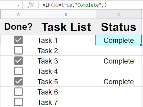
When the checkbox is checked, we will use the IF function to display the word “Complete”. This is done by telling Google Sheets to display the word “Complete” if the cell containing the checkbox is equal to “TRUE”
The formula is this:
=IF(A2=TRUE, “Complete”,)
So if cell A2 = TRUE (if the checkbox is checked), the cell containing the formula (C2) will display the word “Complete”. If cell A2 is NOT equal to TRUE (if the checkbox is unchecked / is FALSE), the formula will display nothing / the cell will be blank.
In the image below, this formula is copied into the cells in column C. So notice that the checkbox in cell A2 is checked, and the word “Complete” appears in cell C2. But in cell A3 the checkbox is unchecked, so cell C3 remains blank.
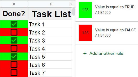
How to use conditional formatting and automatically color code checkboxes
You can use conditional formatting to automatically color checkboxes depending on if they are checked or unchecked.
To color checkboxes with conditional formatting, follow these steps:
- Select the cell(s) that contain the checkbox that you want to apply conditional formatting to
- Click “Format” on the top toolbar
- Click “Conditional formatting”
- Click “Add another rule”
- Choose “Is equal to” from the “Format cells if” dropdown
- Enter the text “TRUE” into the blank field to format cells when the checkbox is checked (Enter “FALSE” to format cells when checkbox is unchecked)
- Select a fill color, text color, or other formatting that you want to apply when the checkbox is checked / unchecked
As you can see in the example image below, when the checkboxes are checked, the cells turn green, and when the checkboxes are unchecked, the cells turn red.
This content was originally created by Corey Bustos / SpreadsheetClass.com
Create an interactive chart by using checkboxes
Checkboxes can also be used to create an interactive chart. This is done by using a formula that interacts with the checkbox, and then connecting the chart to the data that is displayed by that formula.
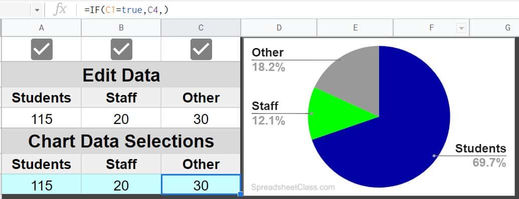
In this example we have a pie chart that shows the distribution of staff, students, and other people at a school. We are going to make it so that our pie chart will only include the data / categories that are associated with a checked checkbox. If the checkbox is checked, the data will show on the chart, if the checkbox is unchecked, the data will not display on the chart.
In this case this is done by entering the data in cell C4, and an IF formula in cell C7. The IF formula will display the data in cell C4 if the checkbox in cell C1 is checked. If the checkbox in cell C1 is unchecked, the IF formula will display nothing and the cell will be blank, which will cause the data to disappear from the pie chart.
Notice in the image directly below, all three categories (Students, staff, other) display on the chart, because all three checkboxes are checked.
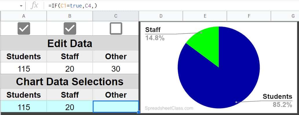
In the image below, notice how the “Other” category does not display on the pie chart because the checkbox for the “Other” category data is unchecked.
Click here to learn how to create charts in Google Sheets.