Copy / paste formatting + using paint format in Google Sheets

In Google Sheets, you can copy formatting from one location in your spreadsheet to another. This is a very handy trick that makes formatting spreadsheets fast, and it allows you to quickly replicate formatting over and over after you spend the time to customize the formatting the first time.

When you copy formatting from one place to another in your spreadsheet, the values and formulas are not copied / pasted, and only the formatting is transferred.

In this lesson I will show you multiple ways to copy formatting in a Google spreadsheet, including the keyboard shortcut, “Paint format”, and the menu option to paste formatting. I’ll also show you the effect that these options have when you select cells vs. entire columns and rows.

Copy / Paste formatting only shortcut

First let’s go over an example of how to use the keyboard shortcut to copy / paste format only. This is the easiest way to copy formatting in your spreadsheet. First you use the normal keyboard shortcut to copy a selection (Ctrl + C for Windows and Command + C for Mac), and then you use a special keyboard shortcut to paste only the formatting, as shown below.

To copy and paste formatting only in Google sheets, follow these steps:

1. Select the cell or range of cells that contains the formatting that you want to copy
2. Press Ctrl + C on the keyboard to copy the selection (Command + C for Mac)
3. Select the cell where you want to paste the formatting into
4. Press Ctrl + Alt + V on the keyboard to paste the formatting only (⌘ + Option + V for Mac)

In this example we have student data in cells that have been formatted in several ways, such as fill color, font size, and bold font.

We are going to copy the formatting from the left side of the sheet, to the right side of the sheet, so that the right side of the sheet is formatted exactly like the left side is. In this case we are going to paste the formatting only, without transferring the values and formulas from the cells.

To do this we will use the keyboard shortcut to copy the cells and then paste format only.

First we select the range A1:C5. Then press Ctrl + C (Command + C for Mac) on the keyboard.

As you can see in the image below, the range A1:C5 has been copied. The blue dotted lines that appear around the range indicate that the selection is copied.

Click here to get your Google Sheets cheat sheet

Cell E1 is selected, which is where we are going to paste the formatting. When you are pasting multiple cells, select the first cell that is in the range that you want to paste into (the cell that is on the top left of the range to be pasted into).

Then press Ctrl + Alt + V on the keyboard to paste only the formatting without the values and the formulas (⌘ + Option + V for Mac)

As you can see in the image below, after using the paste formatting shortcut, the formatting from the range A1:C5 has now been copied into the range A1:G5.

In this case the cells in the range E1:G5 do not contain any values, and initially you can see that the fill color formatting has been transferred. But in the image below you can see that after values are entered into the cells, the text and numbers also match the format from the range A1:C5.

Check out this article if you want to learn how to paste values only, without formulas or formatting.

Formatting a single cell vs. a range of cells vs. columns and rows

You can copy formatting from a single cell to another cell, or from a range of cells to another range of cells.

When using any of the methods in this lesson to copy formatting, when you first select a range of cells before copying the formatting, the same size of range will be affected when you paste the formatting.

If you select a range that is three cells wide by three cells tall, when you copy the formatting from that range to another location in the spreadsheet it will affect a range three cells wide and three cells tall, making it match the original selected range.

As you will learn later in the lesson, if you select entire columns or rows before copying the formatting, when you paste the format the width of the columns and the height of the rows will be transferred as well.

Using paint format to copy formatting

Paint format allows you to click a button on the top toolbar to copy the formatting of a selected range, and then you simply select the cell where you want the formatting to be pasted into and Google Sheets automatically transfers the formatting from the selected range to the desired location.

I often use “Paint format” to copy formatting when I build spreadsheets, such as when I want to create new tabs with the same formatting as an existing tab.

To copy formatting with paint format in Google sheets, follow these steps:

1. Select the cell or range of cells that you want to copy the formatting from
2. Click the paint format button on the top toolbar (the button looks like a paint roller and is beside the print button)
3. Click on the cell where you want to copy the formatting to

After following these steps Google Sheets will automatically transfer the formatting from the selected source location into the specified destination cell / range.

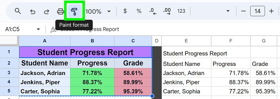
As you can see in the image below, the range A1:C5 is selected, and dotted lines have appeared around the selected range just like when using the keyboard shortcut to copy, but in this case the dotted lines have appeared because the paint format button has been clicked. The paint format button will be highlighted after clicking it, indicating that it is active and that you can now select the cell to copy the formatting into.

As you can see in the image below, the paint format tool has now transferred the formatting from the range A1:C5, to the range E1:G5.

Copying the formatting from one column to another (includes width)

Now let’s go over an example of copying formatting from column to column, where we select an entire column before copying the formatting, rather than selecting just the cells.

When you select entire columns before copying the formatting, the width of the columns will be transferred to the destination columns in addition to the formatting of the cells.

For example, if you select column A, click the paint format button, and then click on column E, not only will the formatting from the cells be transferred to column E… but column E will adjust to the same width as column A.

This is something that I use very often when I have sections of my spreadsheet that I want to replicate exactly into another part of the sheet.

To copy formatting from column(s) to column(s) in Google Sheets, select the column or columns that you want to copy the formatting from, click the “Paint format” button on the top toolbar (looks like a paint roller), and then select the column that you want to transfer the formatting to.

As you can see in the image below, columns A through C have been selected. Not only are the cells highlighted in blue, but the letters of the columns themselves are highlighted, indicating that the entire columns are selected. You can also see that columns E, F, and G are formatted plainly, and have a very narrow column width.

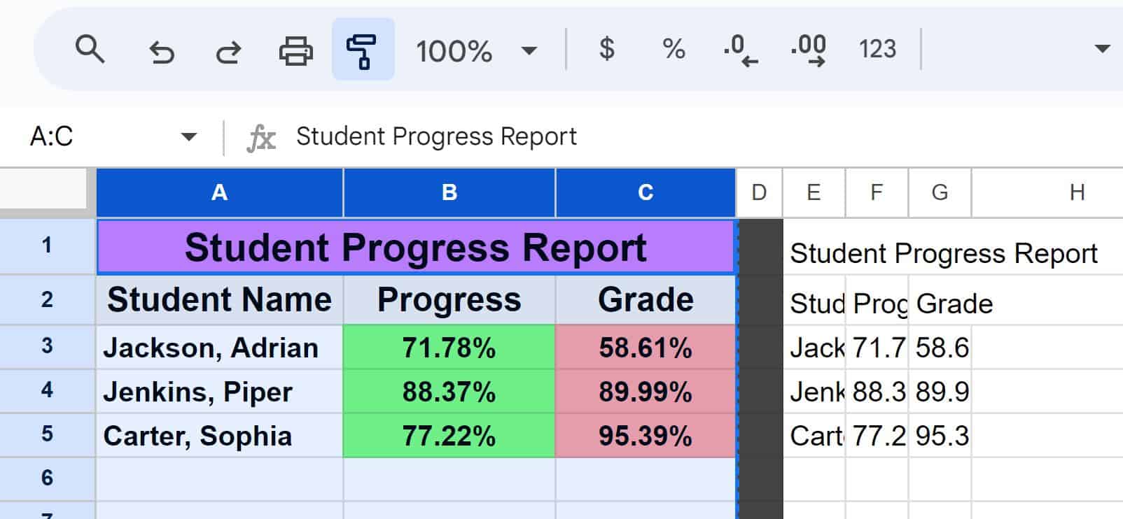
After selecting the columns, we click the “Paint format” button.

Then click on column E, and Google Sheets automatically transfers the formatting from columns A through C, to columns E through G.

As you can see in the image below, the columns that we transferred the formatting into have automatically expanded to match the width of the columns from the original range, and the formatting in the cells such as fill color and font formatting have been transferred as well.

Copying the formatting from one row to another (includes height)

You can also copy formatting from row to row, and the formatting from the rows including the height of the row will be transferred into the chosen location / row(s) in your spreadsheet.

To copy formatting from row(s) to row(s) in Google sheets, select the row or rows that you want to copy formatting from, click the paint format button, and then select the row where you want to copy the formatting to.

As you can see in the image below, rows 3 through 5 are selected.

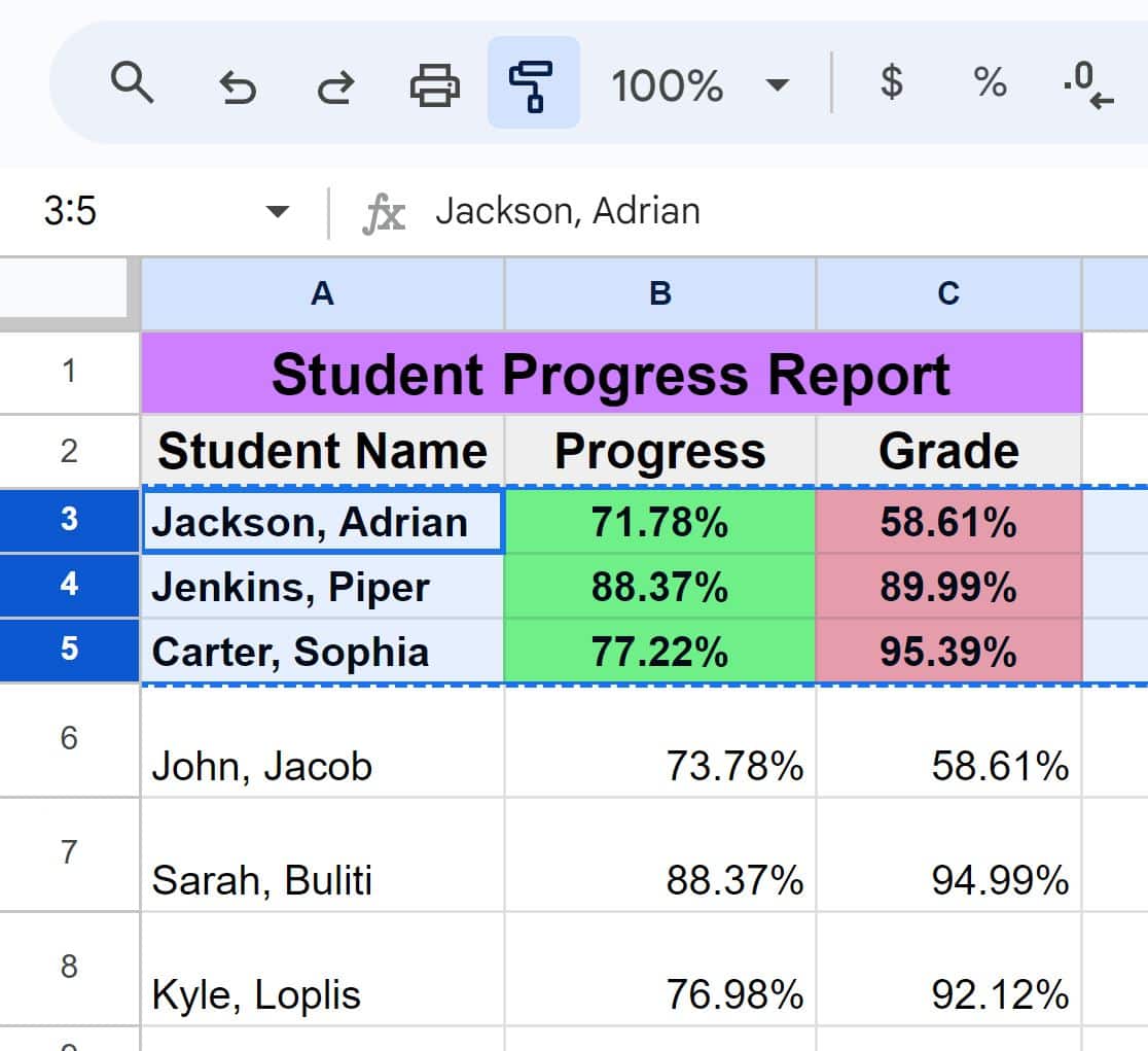
Then we click the paint format button, and the blue dotted lines appear around the selected range.

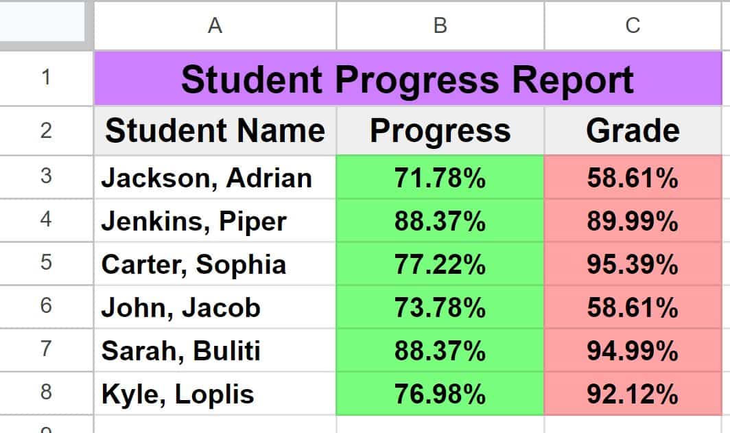
Then we click on row 6, and Google Sheets automatically transfers the formatting from rows 3 through 5, into rows 6 through 8.

This is something that is very handy when you have new data to enter and you want to copy the formatting from the upper rows into the rows below.

Copy the formatting from one sheet to another

Now let’s go over an example of copying the formatting from an entire sheet into a different tab. To do this we will select all of the columns and rows at once, and this means that when we transfer the formatting from one sheet to another, every aspect of the formatting will be copied, including the fill color, text formatting, column width, and row height.

To copy formatting from one sheet to another in Google Sheets, follow these steps:

1. Press Ctrl + A on the keyboard to select all of the rows and columns, or you can click the empty square to the left of column A and above row 1
2. Click the “Paint format” button (looks like a paint roller)
3. Click on the tab that you want to transfer the formatting to, or create a new tab
4. Click on cell A1 in the tab that you want to copy the formatting into

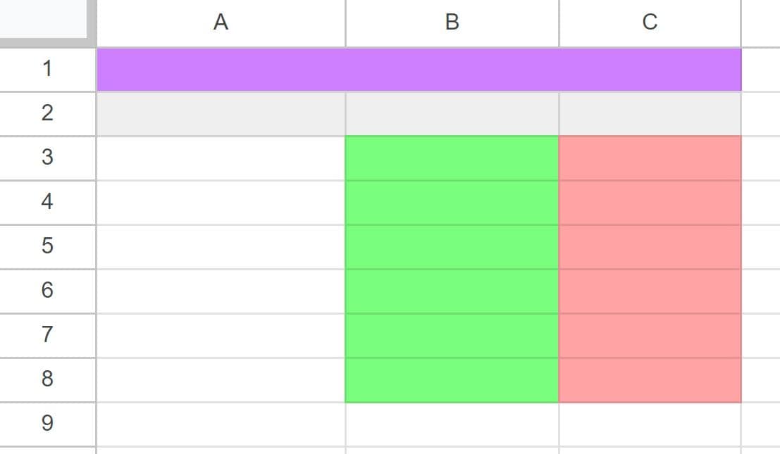
After following these steps, the destination tab will have the exact same formatting as the original tab, including column width and row height.

As you can see in the image below, the entire sheet has been selected, and all of the columns and rows are highlighted.

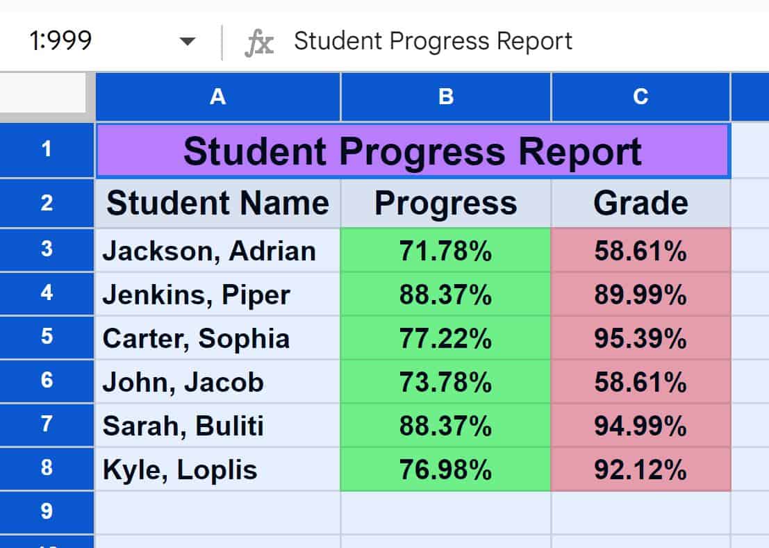
Then we click the paint format button on the top toolbar.

Then click on a different tab, and click on cell A1.

As you can see in the image below, the formatting from the original tab has been copied into another sheet

Using the “Paste special” menu to copy / paste formatting

Now let’s go over how to paste formatting only by using the “Paste special” menu. This is very similar to the keyboard method, except instead of using the shortcut to paste format only, we will right-click and use the menu option.

To copy and paste formatting by using the “Paste special” menu, follow these steps:

1. Select the cell or range of cells that you want to copy the formatting from
2. Press Ctrl + C on the keyboard to copy the selection (Command + C for Mac)
3. Right-click on the cell that you want to copy the formatting to
4. Click “Paste special” and then click “Format only”

As you can see in the image below, just like with the other methods in this lesson, the formatting from the cells has been transferred from one place to another in the spreadsheet.

The image below shows that the range A1:C5 has been selected and copied. E1 is selected which is where we want to paste the formatting.

Then we right-click on cell E1, then click “Paste special”, and then click “Format only”.

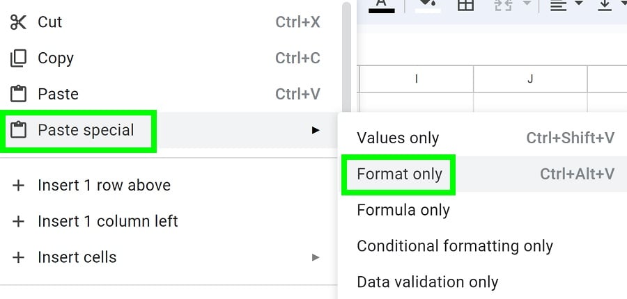
After following these steps, the formatting is copied from the range A1:C5, to the range E1:G5.

Now you know how to easily copy formatting from one place to another in your Google spreadsheets!