
Have you ever encountered the #DIV/0! error while working in Google Sheets? It’s a common issue that happens when dividing in a spreadsheet. This is an error that simply states that the spreadsheet is trying to divide by zero, which is not possible in math and therefore not possible in a spreadsheet.
This is an error that I encounter frequently in my work in a variety of ways, such as when I am creating a formula to average student scores but the data has not been entered yet.
The divide by zero error does not necessarily mean that there is anything wrong with the way your formula is set up. A formula can attempt to divide by zero because you have created a formula but have not entered data yet, or it can mean that your data simply has zero values in it.
In this article, I will show you how to fix or remove the divide by zero error in Google Sheets. We’ll explore how to use the IFERROR function to easily handle this error, understand why the #DIV/0! error occurs when dividing, and how to fix your formula when there is an actual formula error instead of an expected error due to zeros in your data.
To remove the divide by zero error in Google Sheets, follow these steps:
- Select the cell containing the formula that’s causing the #DIV/0! error, such as a division formula like this: =A2/B2
- Apply the IFERROR function to the formula causing the #DIV/0! error, like this: =IFERROR(A2/B2, “N/A”)
After following the steps above, you’ll have effectively removed the divide by zero error in your Google Sheets. The IFERROR function will now display the value or message you specified when a #DIV/0! error occurs. Later I’ll show you different ways to customize the message.
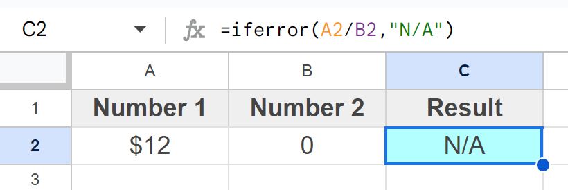
As you can see in the image below, the formula in the cell C2 is dividing cell A2 by cell B2. But cell B2 has a zero in it, and so this means that the formula is trying to divide by zero, which causes a divide by zero error.

The error can be handled by using the IFERROR function, as shown in the image below. After using the if error function, cell C2 now displays the text “N/A” when a #DIV/0! error occurs.
Click here to learn how to divide numbers, cells, rows, and columns in Google Sheets.
Now let’s go over some detailed examples and instructions on how to remove (or fix) the divide by zero error in Google Sheets.
What causes the #DIV/0! error in Google Sheets
The #DIV/0! error can be frustrating if you don’t know what it is. Especially when your formula is set up correctly but the cell displays an error.
The #DIV/0! error in Google Sheets occurs when you attempt to divide a number by zero or an empty cell. A cell that is empty is interpreted by a spreadsheet as having a zero value.
So when you encounter the divide by zero error, again it doesn’t necessarily mean that you entered the formula wrong, it is simply the spreadsheet telling you that there is a zero in the denominator of a formula that you are using. The denominator is the value that is on the bottom of a division equation, or the number that you are dividing by.
Here are the different ways that the error can occur:
- Dividing by zero: The most common cause of the #DIV/0! error is attempting to divide a number by zero. For instance, if you have a formula like “=A1/B1,” and B1 contains a zero value, Google Sheets doesn’t know how to handle it, resulting in the #DIV/0! error.
- Empty cells in the denominator: Another situation that triggers this error is when you try to divide by a cell that is empty. If the cell you’re referencing as the denominator in your division formula is devoid of any value, Google Sheets considers it as zero, leading to the same error.
- Referring to the wrong data: Sometimes the divide by zero error is a legit error when you have referred to the wrong cell or range of cells with your formula. For example, if you meant to average column A but accidentally referred to column B which is empty, the average function would return a divide by zero error.
- Data is missing: If you set up a formula that divides, and it is connected to cells that are missing data, such as when you create a report and have not imported the data yet, the division formula for any function that divides like the average function, will display a divide by zero error if there is a zero value in the denominator due to missing data.
Use IFERROR to handle the divide by zero error in Google Sheets
The IFERROR function is a very useful formula that can help you handle errors from a wide variety of formulas, but here we will focus on using the formula to handle the #DIV/0! error.
The IFERROR function allows us to perform an operation or use a formula, and tell Google Sheets that if an error is encountered, to display the specified criteria. For example, if there is a Formula error, we can display the text “N/A”, or “Error”, or any value that we want.
To use IFERROR to handle the divide by zero error, follow these steps:
- Select the cell that contains the formula that you want to modify to handle the #DIV/0! error
- Modify the formula by incorporating the IFERROR function. Place “IFERROR(” at the beginning of the formula
- Insert the original formula that you want to evaluate
- Type a comma, and specify what should be displayed if the original formula results in an error, like “Error” or “N/A”
- Press “Enter” on the keyboard. The final formula will look like this: =IFERROR(A3/B3, “N/A”)
After following the steps above, you’ll have successfully used the IFERROR function to handle the divide by zero error in your Google Sheets. This means that when the original formula would produce a #DIV/0! error, it will now display the message or value you specified instead.
The Google Sheets IFERROR function description:
Syntax:
IFERROR(“no error”, “error”)Formula summary: “Returns the first argument if it is not an error value, otherwise returns the second argument if present, or a blank if the second argument is absent.”
Let’s say that you have a spreadsheet for tracking expenses. In this example, we have a column for “Total Expenses” and another column for “Number of Transactions.” You want to calculate the average expense per transaction, but sometimes the “Number of Transactions” cell might be empty, leading to the #DIV/0! error.
What we are going to do is use the IFERROR function to make the cell display “N/A” when the “Number of Transactions” is empty.
To do this, we will apply the IFERROR function to the formula calculating the average expense, so it handles the error.
Formula before: =A3/B3
Formula after: =IFERROR(A3/B3, “N/A”)
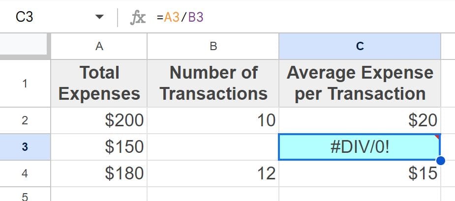
As you can see in the image above, cell C3 is displaying a divide by zero error, because the formula is trying to divide by cell B3, which is empty / zero.
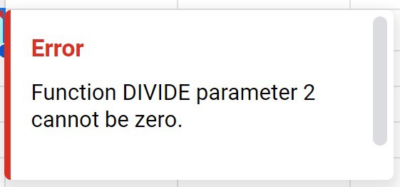
When you hover your cursor over the cell that displays “#DIV/0!”, an error message will pop up that says “Function DIVIDE parameter 2 cannot be zero.”
As you can see in the image below, after applying the if error function to the division formula, cell C3 is now displaying the text “N/A” instead of displaying a #DIV/0! error. This formula can be copied into the other cells in the column so that the formula will handle the error when this happens in any row.
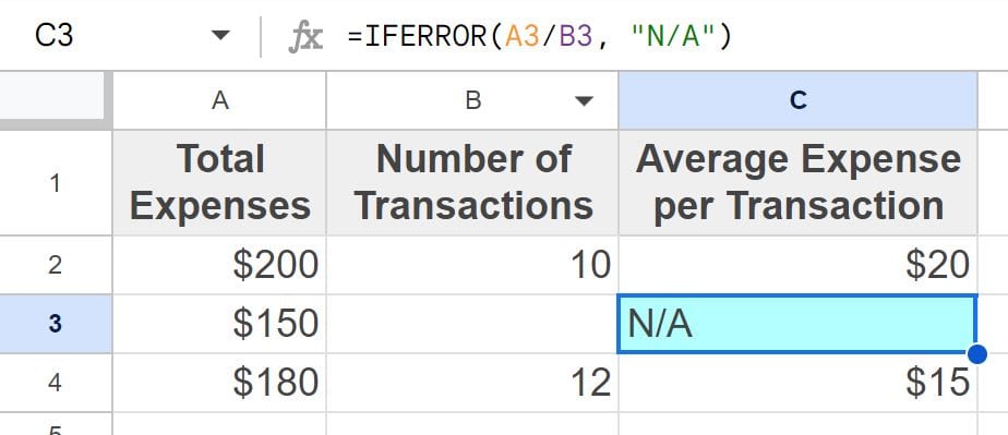
Note that when you put a formula inside of the if error function as demonstrated above, this is called “Nesting” a formula. So we can say that we are “nesting” a division formula inside of the IFERROR function, or we can also say that we are “wrapping” the IFERROR function around the division formula.
#DIV/0! error when using the AVERAGE function in Google Sheets
The AVERAGE function also causes divide by zero errors, because to average you must divide, and when the average function refers to a range that only contains zeros or empty cells, it will display a #DIV/0! error.
To remove the #DIV/0! error when using the AVERAGE function, follow these steps:
- Select the cell that contains the AVERAGE formula that you want to modify to handle the #DIV/0! error
- Modify the formula by incorporating the IFERROR function. Place “IFERROR(” at the beginning of the formula
- Insert the AVERAGE formula that you want to evaluate
- Type a comma, and specify what should be displayed if the original formula results in an error, like “Error” or “N/A”
- Press “Enter” on the keyboard. The final formula will look like this: =IFERROR(AVERAGE(B4:C4),”N/A”)
After following the steps above, you will have removed the #DIV/0! error. Instead of displaying the error message, your cell will show the value or message you specified.
Let’s say that you have data that shows the scores from two different tests for a list of students. In this example, we want to find the average between both tests, for each student. However, for some students, there might be no data recorded, resulting in the #DIV/0! error.
What we are going to do is use the AVERAGE function with the IFERROR function to make the cell display “N/A” when there are no values in the selected range.
To do this, we will use the AVERAGE function to calculate the average test score, and nest it within the IFERROR function to handle the error exactly like we want.
Formula before:
=AVERAGE(B4:C4)
Formula after:
=IFERROR(AVERAGE(B4:C4),”N/A”)
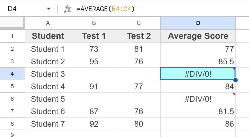
As you can see in the image above, cell D4 is displaying a divide by zero error, because the formula is trying to take the average of cells B4 and cell C4, both of which are blank. This causes an error because the AVERAGE function is trying to divide by blank cells / cells with a zero value.
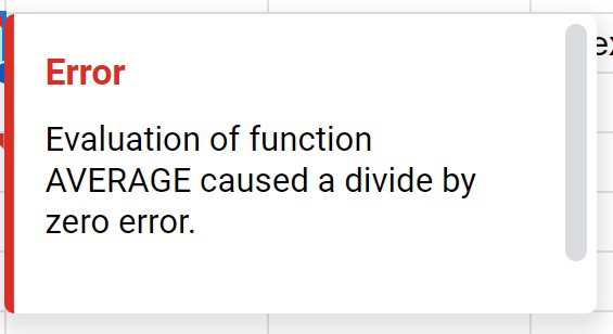
When you hover your cursor over the cell that displays “#DIV/0!”, an error message will pop up that says “Evaluation of function AVERAGE caused a divide by zero error.”
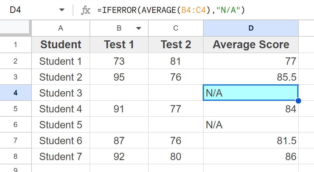
As you can see in the image below, after applying the IFERROR function to the AVERAGE function (wrapping IFERROR around the AVERAGE function), cell D4 is now displaying the text “N/A”
Different ways to handle the error
With the IFERROR function, you can display any text/value that you want when a formula error occurs. You can choose to display text such as “Error”, or you can display the number 0, or you can tell Google Sheets to leave the cell blank.
Display a blank cell instead of text when there is an error
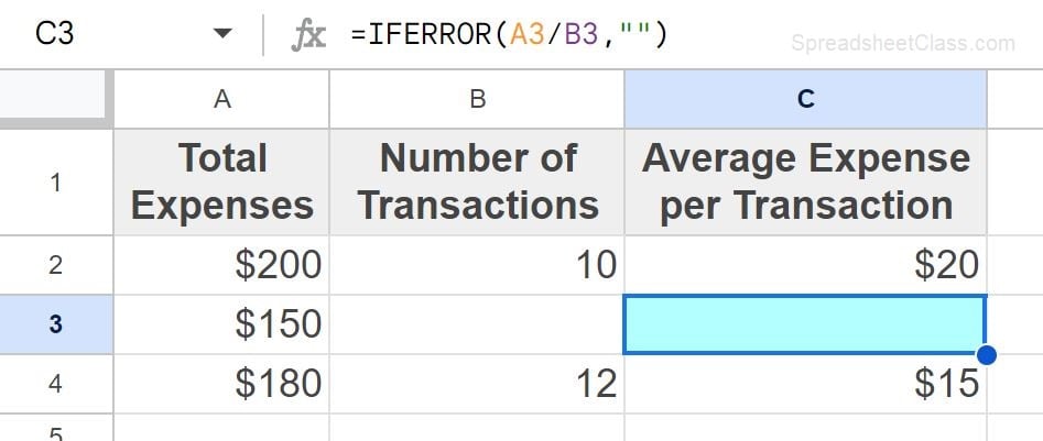
If you want to leave the cell blank when a formula error occurs, there are multiple ways to express this with the IFERROR function. Three ways to do this are shown below.
You can specify “Blank” with two quotation marks, or you can simply leave the criteria empty after typing the comma in the formula, or you can simply leave the comma and the criteria out altogether, since the IFERROR function will display a blank cell by default if criteria is not specified for the error message.
=IFERROR(A3/B3,)
=IFERROR(A3/B3)
=IFERROR(A3/B3,””)
Display a text when there is an error
The two formulas below demonstrate how to specify customized text for the error message in the IFERROR function.
=IFERROR(A3/B3, “N/A”)
=IFERROR(A3/B3, “Error”)
Display a number when there is an error
The formula below demonstrates how to specify a number when an error occurs in the IFERROR function.
=IFERROR(A3/B3, 0)
Fixing the formula when the error is not expected
Sometimes a divide by zero error can arise when you set up your formula incorrectly, such as referring to the wrong cell or the wrong range of cells.
For example, if you enter the formula =AVERAGE(G1,G2) and get a divide by zero error, when you know there should not be an error due to zeros in the data, check closely to make sure that you are referring to the correct cells. If you discover that you mean to refer to cells H1 and H2, and that cells G1 and G2 are blank, this would be the cause of the error and can be fixed by changing the formula to the correct references like this: =AVERAGE(H1,H2)
Error when dividing by the SUM function / other functions
Another way that the divide by zero error can occur, is when you are using other functions in the denominator of your formula, such as when you are dividing by the result of the SUM function.
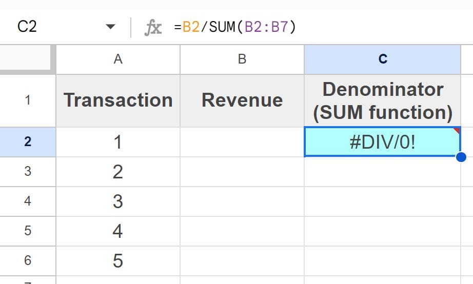
As you can see in the image below, cell C2 is dividing cell B2 by the SUM function (which is summing column B).
And no data is entered into column B and the cells are blank, this means that the result of the sum function is zero, which means that the division formula is trying to divide by zero, causing a #DIV/0! error.
=B2/SUM(B2:B7)
Fixing the error by entering data into blanks cells
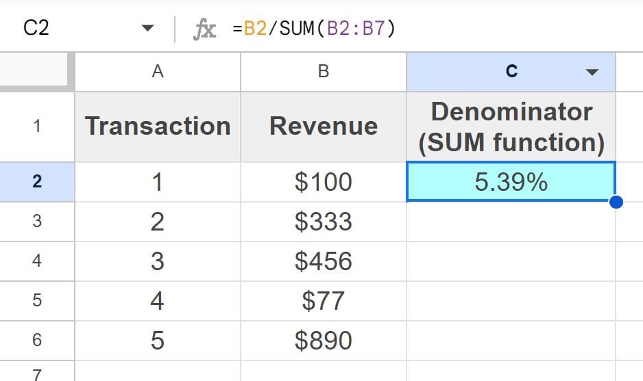
In this case, instead of removing the divide by zero error with the IFERROR function, we are going to fix the #DIV/0! error by entering data into the empty cells.
As you can see in the image below, cell C2 now displays the result of the division formula, because the numbers have been entered into column B, and the denominator of the division formula is no longer zero.
Now you know exactly how to handle the divide by zero error when you encounter it in Google Sheets, whether you want to display a custom message when the error occurs, or if you want to fix the error by either fixing your formula or filling in missing data.

