
In Google Sheets you will sometimes have the need to calculate the amount of time between two different times (time difference), such as when you want to calculate how long a job shift is, or when you want to calculate the time that has elapsed given two times. This can be done very easily by subtracting one time value from another, but the trick is to make sure that the cells are formatted so that the times that you enter are displayed correctly, and so that the calculated duration also displays in the correct format.
For example, if you enter the time 7:00 PM in cell B2, and the time 1:00 PM in cell B1, and then subtract cell B1 from cell B2, the formula will display that 6 hours (6:00:00) are between the first and second time. But you need to make sure that the cell that contains the formula is in “Duration” format for the calculated duration to display properly.
To calculate the duration between two times in Google Sheets, follow these steps:
- Type an equals sign (=)
- Type the address of the cell that contains the more recent / larger time value
- Type of minus sign (-)
- Type the address of the cell that contains the older / smaller time value
- Press “Enter” on the keyboard. The final formula will look like this, where cell B2 is the more recent time, and cell B1 is the older time: =B2-B1
- Select the cell that contains the formula, click the “More formats” menu on the top toolbar (The button that says “123”), and then click “Duration”
After following these steps the cell that contains the formula will display the time / duration that is between the two time values.
Calculating the number of days between dates is similar to calculating the duration between times, but there are important differences and additional methods to learn, so click here to learn how to calculate the number of days between dates.
Finding the duration between two times
Let’s go over an example of calculating the time / duration between two times, where there is not a date included with the time value.
As you can see in the image below, the time 8:30 AM. is entered into cell A2, and the time 5:00 PM. is entered into cell B2.
The formula in cell C2, subtracts cell A2 from cell B2, which gives an answer of 8 hours and 30 minutes (8:30:00). So there are 8 hours and 30 minutes between 8:30 AM and 5:00 PM, or in other words 8 hours and 30 minutes elapsed between the two given times.
=B2-A2

Further below I will show you detailed instructions on making sure that the cells are in the correct format.
Finding the duration between two dates / times
Now let’s go over an example of calculating the time difference between two dates with time values included. This will allow us to calculate the time that has elapsed between two dates / times.
As you can see in the image below, the date/time 11/1/2023 8:30 AM is entered into cell A2, and the date/time 11/3/2023 5:00 PM is entered into cell B2.
We are going to calculate the time that is between these two date/time values, by subtracting cell A2 from cell B2.
=B2-A2

As you can see in the image above, the formula in cell C2 has calculated the amount of time between both date/time values, which is 56 hours and 30 minutes (56:30:00).
Notice how in this particular case, by default the spreadsheet gives a number/decimal value, but after converting the cell to duration format, the duration/time displays correctly (shown in cell C3).
Formatting the times and durations correctly
Now let’s go over how to properly format the cells when calculating that duration between two times.
First, we will make sure that the time values to be calculated are displayed in “Time” format.
Then we will make sure that the calculated duration displays in “Duration” format.
The image below shows two time values that have been entered into cell A2 and cell beat you, with the intention of subtracting the time 5:00 PM From the time 8:30 AM. However, as you can see in the image, cell B2 displays “5:00” but when it is selected the formula bar shows that the actual time entered is 5 AM. This is why it is important to display the values in “Time” format, so that you are certain whether each time value is AM or PM.
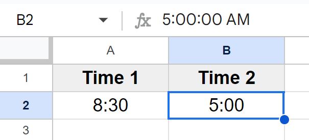
When typing a time value into a spreadsheet cell, make sure that you include “AM” or “PM” so that the spreadsheet does not automatically choose one for you which can sometimes cause confusion as mentioned above. If you want to specify the time “8:30 a.m.” then type the time like this: 8:30 AM
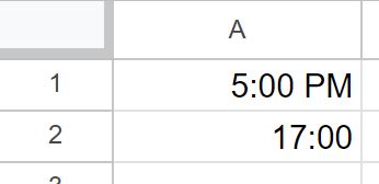
In an image below, you can see an example of the format that a time value sometimes displays in, when the cell is not in “Time” format, even when you correctly specify AM / PM. The time “5:00 PM” has been typed into the cell, but the cell is displaying “17:00” which is the military time equivalent to 5:00 p.m.
To change cells to “Time format, follow these steps:
- Select the cell or cells that you want to convert to “Time” format
- Click the “More formats” menu on the top toolbar (The button that says “123”)
- Click “Time”

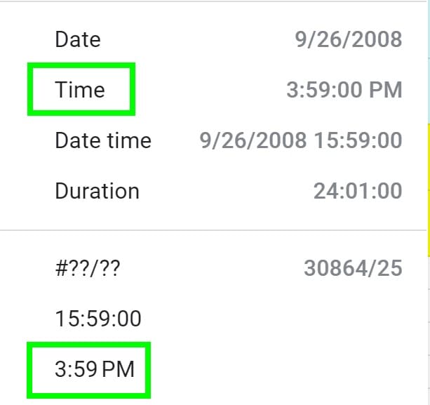
After selecting the cells with the time values, first click the “More formats” menu, (as shown in the image above), and then click “Time” (as shown in the image below).
If your time values are attached to dates, you can select the format “Date time” to display both the date and the time.
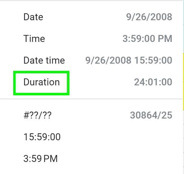
Then select the cell that contains the formula, and change the cell format to duration format by clicking the “More formats” menu and then click “Duration”.
Now you can easily calculate the amount of time (duration) that is between two dates in Google Sheets.

