
If you have values in your spreadsheet that are displaying in date format when you do not want them to, there are multiple ways to remove the date formatting. This happens often when you enter data into a column that was previously formatted for dates, and sometimes it even seems to happen randomly where a number turns into a date.
In this lesson I will show you multiple ways to remove date formatting, depending on your situation and preferences.
Click here if you want to learn how to change / customize date formats instead of removing the date format.
To remove date formatting in Google Sheets, follow these steps:
- Select the cells with date formatting
- Click “More formats” on the top toolbar (The button says “123”)
- Choose any format other than a date format, such as “Number”, “Plain text”, or “Automatic” (Choose the option that best fits your data)
Now let’s go over some examples of the different ways to remove date formatting.
Change the format to “Number”
The most common setting that I use to remove date formatting, is “Number” format. Dates are simply values / numbers displayed in a specific format. Sometimes your numbers will display as a date when you don’t want them to, or sometimes you’ll simply want to see the number values that each date represents.
To change cells to number format in Google Sheets, follow these steps:
- Select the cells that you want to format as numbers
- Click “More formats” on the top toolbar (The button says “123”)
- Click “Number”
In this example we have a list of numbers, but one of the numbers in the list is displayed as a date (as shown in the image below). We want to remove the date formatting so that the value displays as a number.
Although in this case there is only one date in the list, it is good practice to format the entire column / range of data so that it does not happen again and so that any / all instances will be formatted correctly all at once.
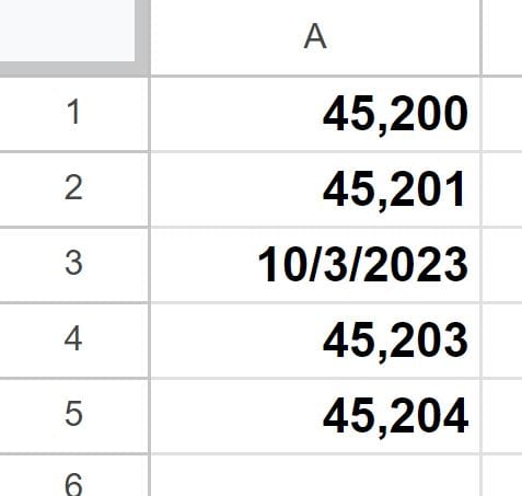
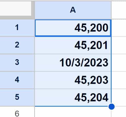
First we will select the cells that contain the values to remove the date formatting from.
Either select the entire column by clicking the letter at the top of the column…
Or select a range by clicking on the first cell in the range, then hold your click and drag your cursor until the desired cells are selected (then release your click).
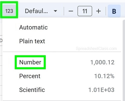
Then on the top toolbar, click the button that says “123”. When you hover your cursor over the button it will say “More formats”.
Then click “Number”
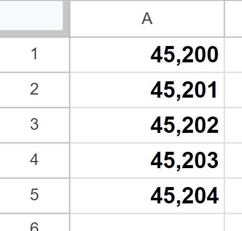
As you can see in the image below, after changing the cells in column A to “Number” format, all of the cells are now showing numbers instead of dates.
Learn about the ultimate formulas cheat sheet
Change the format to “Plain text”
In some cases you may want to remove date formatting by changing cells to “Plain text” format, instead of number format. This is useful for when you want to enter dates as text (such as “Oct 1”) without Google Sheets changing it to an actual date. I do this all of the time when I am making lists with dates.
To change cells to plain text format in Google Sheets, follow these steps:
- Select the cells that you want to format as plain text
- Click “More formats” on the top toolbar (The button says “123”)
- Click “Plain text”
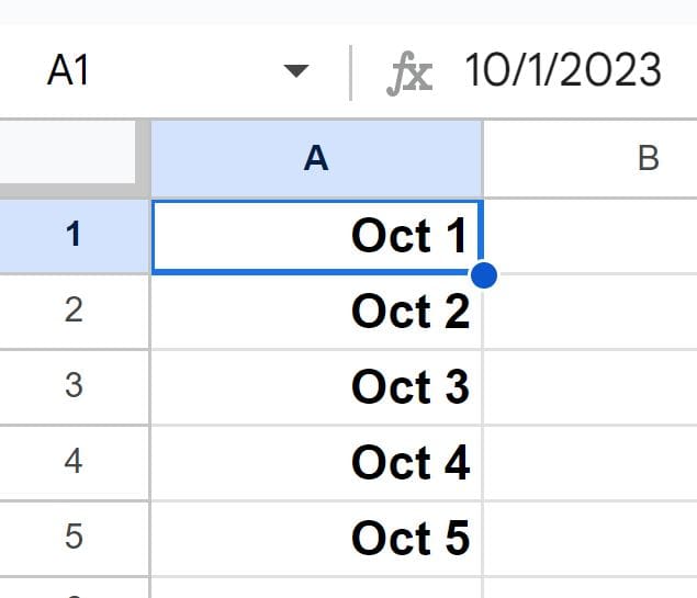
In this example we have a list of dates that were typed as text (Oct 1, Oct 2, etc.) but Google Sheets turned them into dates and is not considering the values entered as text. We can change this by converting the column / cells to plain text.
As you can see in the image below, although the date was typed like this “Oct 1”, in the formula bar you can see that Google Sheets is interpreting it as the date 10/1/2023.
Also notice that the values entered were aligned to the right by default, which is another indication that Google Sheets is interpreting the entered values as dates instead of plain text. We want Google Sheets to interpret it as plain text.
First select the column or the range of cells to format.
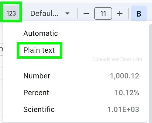
Then click the “More formats” menu on the top toolbar (The button that says “123”), and then click “Plain text”.
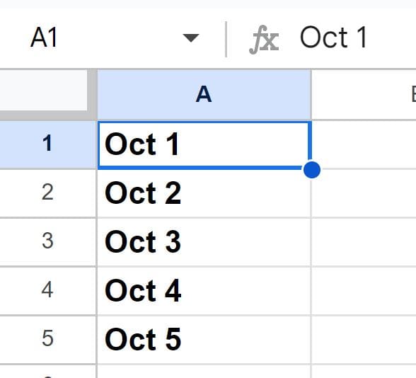
As you can see in the image below, after changing the cells in column A to “Plain text” format, all of the values in the cells are aligned to the left, and the values in the formula bar match what is displayed in the cell, indicating that Google Sheets is now interpreting the values as plain text.
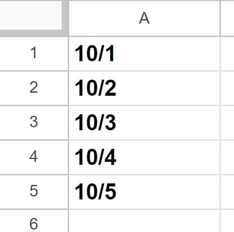
Below is another example that shows dates in the format like this “10/1”, that have been converted to plain text. Again notice that the values are aligned to the left after being turned into plain text.
Change the format to “Automatic”
Another format that you can choose when you want to remove date formatting, is “Automatic”. This is what I choose to reset the format to default. When you have dates that are already entered into the cells, you can choose this format to turn them into plain numbers without commas.
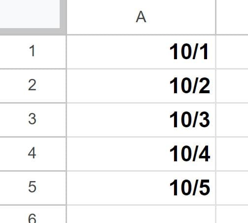
In this example we have a list of dates, and we want to remove the date formatting by changing them into plain numbers / values without commas.
First select the cells / column that you want to format.
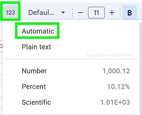
Click the “More formats” menu on the top toolbar (The menu button says “123”).
Then click “Automatic”
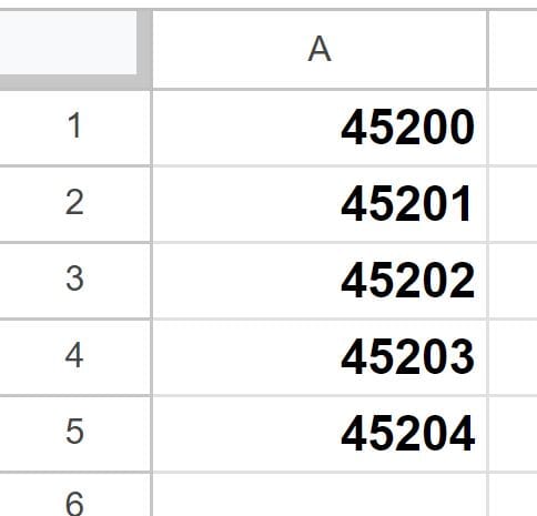
As you can see in the image below, after changing the cells in column A to “Automatic” format, all of the cells are now showing plain numbers / values instead of dates.
Note that if you are referring to a date with a formula, and you format the cell with the formula as “Automatic”, the value will remain in the format of cell that you are referring to, since Google Sheets is automatically detecting the format from the original cell.
So if a date is in cell A1, and cell A2 has this formula “=A1″… and you set cell A2 to “Automatic” format, cell A2 will still display as a date. This is where you can simply choose “Number” or “Plain text” to assure that the date formatting is removed and that the value displays how you want it to.
Now you know how to remove date formatting from cells / values in Google Sheets!
Check out this lesson if you want to learn how to add days, month, or years to a date in Google Sheets.

