If you have numbers in your Google spreadsheet that you need to round, this lesson will teach you all of the different ways to round numbers in a spreadsheet.
I will teach you how to round to the nearest whole number, how to round up or down to a specified decimal place, how to round to the nearest 10 or nearest 100, and more.
First we will go over how to use the ROUND function to round numbers according to traditional mathematical rules, where the formula decides to round up or down based on whether the next highest or the next lowest number is closer.
Then I’ll show you how to use the ROUNDUP function to ensure that you round up, and then we’ll go over how to use the ROUNDDOWN function to ensure that you round down.
When you see words like “tenth” and “hundredth” we are talking about decimal places (when there is a “th” at the end of the word.)
- Hundreds: 100, 200, etc.
- Tens: 10, 20, etc.
- Whole numbers: 1, 2, etc.
- Tenths (1 decimal place): 0.1, 0.2, etc.
- Hundredths (2 decimals places): 0.01, 0.02, etc.
Positive vs. Negative decimal place criteria: If you use a positive number to specify the number of decimal place criteria in the ROUND / ROUNDUP / ROUNDDOWN function, this will specify how many decimal places to round to. If you use a negative number to specify the decimal place criteria, this will indicate multiples of 10 to round to.
- 2 = 2 decimal places (hundredths)
- 1 = 1 decimal place (tenths)
- 0 = no decimals / whole number
- -1 = tens
- -2 = hundreds
Using the ROUND function
First let’s go over how to use the ROUND function, which will round according to the ordinary rounding rules, where the number will be rounded up if it is closer to the number above it, and the number will be rounded down if it is closer to the number below it. If the number is halfway between the number that is above and below it, the formula will round up.
With the round function, you simply specify the number to be rounded, and then specify the number of decimal places that you want to round to.
To round a number in Google Sheets, follow these steps:
- Type =ROUND( to begin the formula
- Type the number to be rounded, or the cell address that contains the number to be rounded
- Type a comma, and then enter a number to represent the number of decimal places to round to
- Press “Enter” on the keyboard. The final formula will look like this: =ROUND(A1,2)
After following the steps above, the number will be rounded according to normal rounding rules.
The Google Sheets ROUND function description:
Syntax:
ROUND(value, [places])Formula summary: “Rounds a number to a certain number of decimal places according to standard rules.”
How to round to the nearest whole number
If you want to round to the nearest whole number, you can use the ROUND function without specifying the number of decimal places to round to, and by default the formula will round to the nearest whole number. Or you can specify “0” decimal places in the formula criteria. I will show you both of these formulas below.
Whole numbers are simply numbers without a decimal, like this: 1, 2, 3, 4, 5…
In this example, we have entered the number “1.5” into cell A2, and cell B2 rounds the number in cell A2 to the nearest whole number, with the formula below. Both of the formulas listed below do the same thing.
The first formula does not specify the number of decimal places, and so the ROUND function defaults to zero decimal places. The second formula specifies zero decimal places, which yields the same result.
=ROUND(A2)
=ROUND(A2,0)
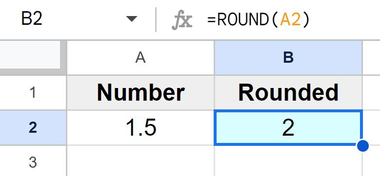
As you can see in the image above, cell B2 displays the number “2”, after rounding the number in cell A2 (1.5) to the nearest whole number.
Since “1.5” is right in the middle of the numbers “1” and “2”, the number was rounded up, which is the traditional rule when rounding a number that lies halfway between the next highest number and the next lowest number.
Rounding two decimal places to the nearest hundredth / cent
In this example, we are going to round to the nearest hundredth, which is the nearest cent when dealing with money/currency. This means that we will round to 2 decimal places.
Hundredths are increments like this: 0.01, 0.02, 0.03, 0.04, 0.05…
In this example, we have entered the number “1.577” into cell A2, and cell B2 rounds the number in cell A2 to 2 decimal places (nearest hundredth), with the formula below.
=ROUND(A2,2)
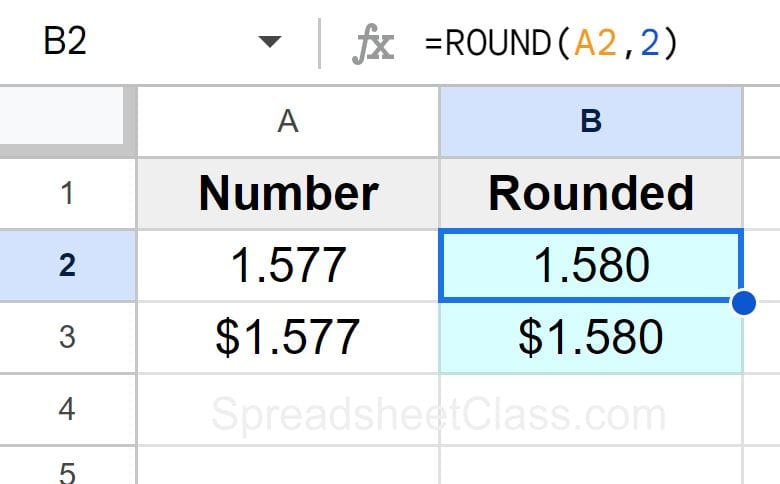
As you can see in the image above, cell B2 displays the number “1.58”, after rounding the number in cell A2 (1.577) to 2 decimal places.
Since “1.577” is closer to “1.58” than it is to “1.57”, the number was rounded up. If the number in cell A2 was “1.573”, the formula would have rounded down to “1.57”.
Round to the nearest tenth (1 decimal place)
To round to the nearest tenth in Google Sheets, round to one decimal place with the ROUND function, like this: =ROUND(A2,1)
For example, if the number “1.57” is entered into cell A2, then the formula below will round the number up to 1.6.
=ROUND(A2,1)
Since “1.57” is closer to “1.6” than it is to “1.5”, the number will be rounded up. If the number in cell A2 was “1.53”, the formula will round down to “1.5”.
Rounding to the nearest ten
If you want, instead of rounding to a number of decimal places or to whole numbers, you can round in multiples of 10. In this example we will round to the nearest ten.
To do this, we will specify the number “-1” as the number of decimal places in the ROUND function.
Tens are increments like this: 10, 20, 30, 40, 50…
In this example, we have entered the number “7” into cell A2, and cell B2 rounds the number in cell A2 to the nearest multiple of ten, with the formula below.
=ROUND(A2,-1)
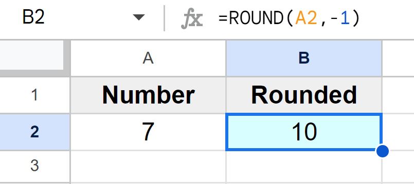
As you can see in the image above, cell B2 displays the number “10”, after rounding the number in cell A2 (7) to the nearest ten.
Since “7” is closer to “10” than it is to “0”, the number was rounded up. If the number in cell A2 was “3”, the formula would have rounded down to “0”.
Rounding to the nearest hundred
In this example, we are going to round to the nearest hundred.
Hundreds are increments like this: 100, 200, 300, 400, 500…
In this example, we have entered the number “77” into cell A2, and cell B2 rounds the number in cell A2 to the nearest multiple of hundred, with the formula below.
=ROUND(A2,-2)
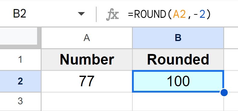
As you can see in the image above, cell B2 displays the number “100”, after rounding the number in cell A2 (77) to the nearest hundred.
Since “77” is closer to “100” than it is to “0”, the number was rounded up. If the number in cell A2 was “33”, the formula would have rounded down to “0”.
Using the ROUNDUP function
Now let’s use a different formula, which will always round up. The ROUNDUP function will round numbers to a specified number of decimal places, but the formula always rounds up to the nearest specified decimal place.
To round up in Google Sheets, follow these steps:
- Type =ROUNDUP( to begin the formula
- Type the number to be rounded up, or the cell address that contains the number to be rounded up
- Type a comma, and then enter a number to represent the number of decimal places to round up to
- Press “Enter” on the keyboard. The final formula will look like this: =ROUNDUP(A1,2)
The Google Sheets ROUNDUP function description:
Syntax:
ROUNDUP(value, [places])Formula summary: “Rounds a number to a certain number of decimal places, always rounding up to the next valid increment.”
Rounding up to the nearest whole number
In this example, we are going to round up to the nearest whole number. To do this we will use the ROUNDUP function, and we will specify zero decimal places, or you can leave out the decimal place criteria and the formula will default to rounding up to the nearest whole number.
In this example, we have entered the number “1.3” into cell A2, and cell B2 rounds the number in cell A2 up to the nearest whole number by using the formula below. Both of the formulas below do the same thing.
=ROUNDUP(A2)
=ROUNDUP(A2,0)
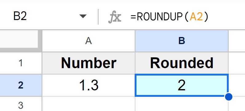
As you can see in the image above, cell B2 displays the number “2”, after rounding the number in cell A2 (1.3) up to the nearest whole number.
Since “2” is the next whole number higher than “1.3”, the number was rounded up to “2”. Notice how the formula rounded up, even though “1.3” is closer to “1” than it is to “2”, because the ROUNDUP function always rounds up.
Rounding up two decimal places to the nearest hundredth / cent
In this example, we are going to round up to the nearest hundredth, which means rounding up to the nearest cent when dealing with money/currency. This means that we will round up, to 2 decimal places.
In this example, we have entered the number “1.333” into cell A2, and cell B2 rounds the number in cell A2 up to 2 decimal places (nearest hundredth), with the formula below.
=ROUNDUP(A2,2)
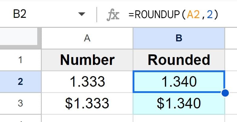
As you can see in the image above, cell B2 displays the number “1.34”, after rounding the number in cell A2 (1.333) up to 2 decimal places.
Since “1.34” is the next “hundredth” increment higher than “1.333”, the number was rounded up to “1.34”.
Using the ROUNDDOWN function
Now let’s use a different formula, which will always round down. The ROUNDDOWN function will round numbers to a specified number of decimal places, but the formula always rounds down to the nearest specified decimal place.
To round down in Google Sheets, follow these steps:
- Type =ROUNDDOWN( to begin the formula
- Type the number to be rounded down, or the cell address that contains the number to be rounded down
- Type a comma, and then enter a number to represent the number of decimal places to round down to
- Press “Enter” on the keyboard. The final formula will look like this: =ROUNDDOWN(A1,2)
The Google Sheets ROUNDDOWN function description:
Syntax:
ROUNDDOWN(value, [places])Formula summary: “Rounds a number to a certain number of decimal places, always rounding down to the next valid increment.”
Rounding down to the nearest whole number
In this example, we are going to round down to the nearest whole number. To do this we will use the ROUNDDOWN function, and we will specify zero decimal places, or you can leave out the decimal place criteria and the formula will default to rounding down to the nearest whole number.
In this example, we have entered the number “1.7” into cell A2, and cell B2 rounds the number in cell A2 down to the nearest whole number by using the formula below. Both of the formulas below do the same thing.
=ROUNDDOWN(A2)
=ROUNDDOWN(A2,0)
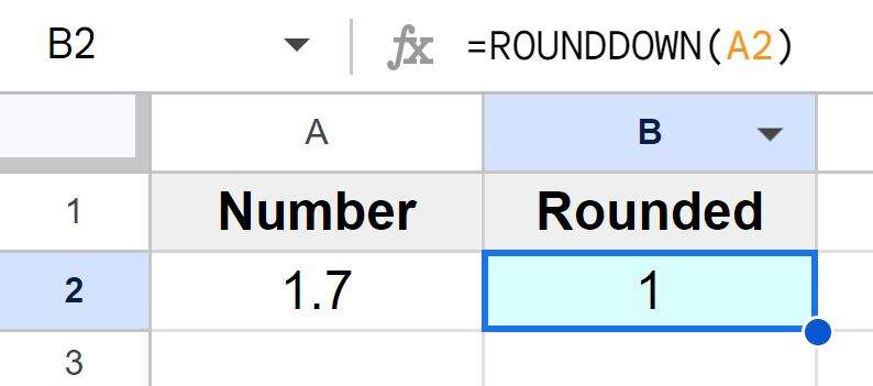
As you can see in the image above, cell B2 displays the number “1”, after rounding the number in cell A2 (1.7) down to the nearest whole number.
Since “1” is the next whole number lower than “1.7”, the number was rounded down to “1”. Notice how the formula rounded down, even though “1.7” is closer to “2” than it is to “1”, because the ROUNDDOWN function always rounds down.
Rounding down two decimal places to the nearest hundredth / cent
In this example, we are going to round down to the nearest hundredth, which means rounding down to the nearest cent when dealing with money/currency. This means that we will round down, to 2 decimal places.
In this example, we have entered the number “1.119” into cell A2, and cell B2 rounds the number in cell A2 down to 2 decimal places (nearest hundredth), with the formula below.
=ROUNDDOWN(A2,2)
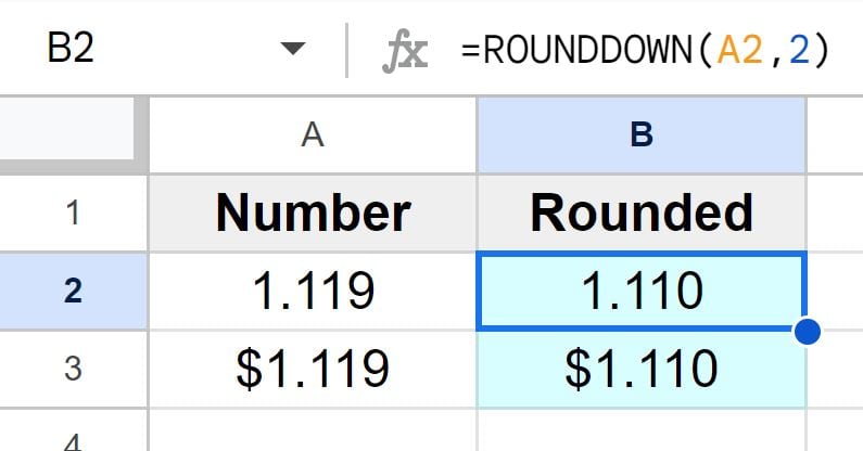
As you can see in the image above, cell B2 displays the number “1.110”, after rounding the number in cell A2 (1.119) down to 2 decimal places.
Since “1.110” is the next whole number lower than “1.119”, the number was rounded down to “1.110”.
As you can see in the example, row 3 displays the same values in “Currency” format, so that you can see how the function works when dealing with currency / money.
You might have noticed that when you click the decrease decimal places button to remove decimal places from a number in your spreadsheet, although the cell displays fewer decimal places and the appears to be rounded, the actual number is still in the background, so if you want to round a number properly, use the instructions in this article to round numbers with formulas. But if you want a number to appear as being rounded while still keeping the exact number in the background, you can decrease decimal places.

