If you want to both sort and filter your data with a single formula in Google Sheets, you can do this by combining the SORT function with the FILTER function.
In this article I will show you multiple ways of combining these two formulas so that you can sort and filter with a single formula, as well as have the ability to sort by multiple columns and filter by multiple conditions, in a single formula.
To sort and filter your data in a single formula, follow these steps:
- Start by typing your filter formula, like this: =FILTER(A3:C,C3:C=”Text”)
- Then use your filter function as the range for a sort function like this: =SORT(FILTER(A3:C,C3:C=”Text”), 1, true)
Using the SORT and FILTER functions in Google Sheets is similar to using it in Excel, but there are some differences between the two. Click here to read the Excel version of this article
SORT FILTER formulas in Google Sheets:
Sort and filter
- =SORT(FILTER(A3:C,C3:C=”Text”),1,true)
Sort by multiple columns and filter by one condition
- =SORT(FILTER(A3:C,C3:C=”Text”),2,true,1,true)
Sort by one column and filter by multiple conditions
- =SORT(FILTER(A3:C,(C3:C=”Text”)+(B3:B>0.5)),2,true)
Sort by multiple columns and filter by multiple conditions (AND logic)
- =SORT(FILTER(A3:C,C3:C=”Text”,B3:B>0.5),2,true,1,true)
Sort by multiple columns and filter by multiple conditions (OR logic)
- =SORT(FILTER(A3:C,(C3:C=”Text”)+(B3:B>0.5)),2,true,1,true)
Click here to get your Google Sheets cheat sheet
Or click here to take the dashboards course
The video below will show you how to use SORT and FILTER functions, individually, and combined!
SORT / FILTER nested formula
The formulas in this lesson are what are called “nested formulas”, which means that we are using / nesting one function “inside” of another function, all within the same Google Sheets formula.
When formulas are nested, you may sometimes hear someone refer to the formula that has another formula nested inside of it, as being the formula that is “wrapped” around the nested formula. For example in the formula below, the FILTER function is nested inside of the SORT function, and conversely the SORT function is “wrapped” around the FILTER function.
You can use the output of your filter function as your sort function range like this: =SORT(FILTER(A2:B,C2:B=100″), 2, false)
This article focuses on combining the SORT and FILTER functions, but if you want to learn how to use them separately, check out the articles linked below:
Sort and filter formula example
Here is a basic example of using the SORT function with the FILTER function in Google Sheets.
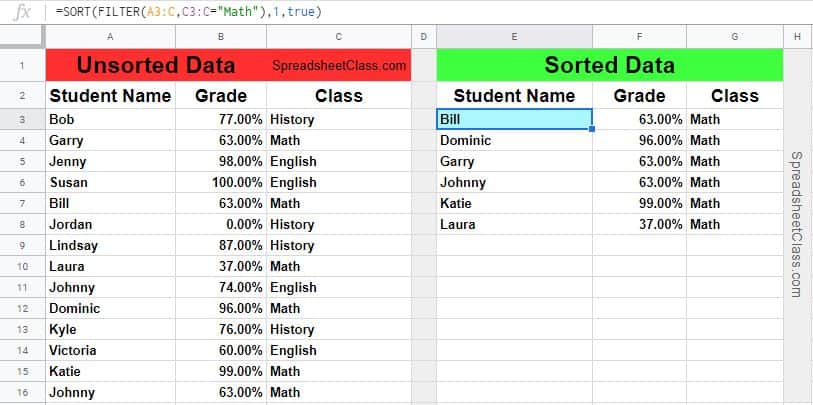
Below is example student data that shows the student’s name, and their grades in multiple classes. We will both filter and sort the data with a single formula.
The task: Filter the student data to show only math classes, and sort the result by student name in ascending order
The logic: Filter the range A3:C, where C3:C is equal to the text “Math”, and then sort by column 1
The formula: The formula below, is entered in the blue cell (E3), for this example
=SORT(FILTER(A3:C,C3:C=”Math”),1,true)

Note that both of the formulas below do the same thing, since the default for the SORT function is to sort by the first column in ascending order if criteria is not specified for the SORT function.
=SORT(FILTER(A3:C,C3:C=”Math”),1,true)
=SORT(FILTER(A3:C,C3:C=”Math”))
Sort by multiple columns and filter by multiple conditions (AND logic)
In this example I will show you how to use the SORT function with the FILTER function, while sorting by multiple columns and filtering by multiple conditions.
In this example we will use “AND logic” for the filter criteria, meaning that both of the filter conditions must be true to be included in the filter output. This is accomplished by separating the filter conditions with a comma.
The task: Filter the student data to show math classes that are above 50%, and sort the result by grade and then by student name, both in ascending order
The logic: Filter the range A3:C, where C3:C is equal to the text “Math”, and where B3:B is greater than 0.5. Then sort the result by column 2 in ascending order, and then by column 1 in ascending order
The formula: The formula below, is entered in the blue cell (E3), for this example
=SORT(FILTER(A3:C,C3:C=”Math”,B3:B>0.5),2,true,1,true)

This content was originally created by SpreadsheetClass.com
Sort by multiple columns and filter by multiple conditions (OR logic)
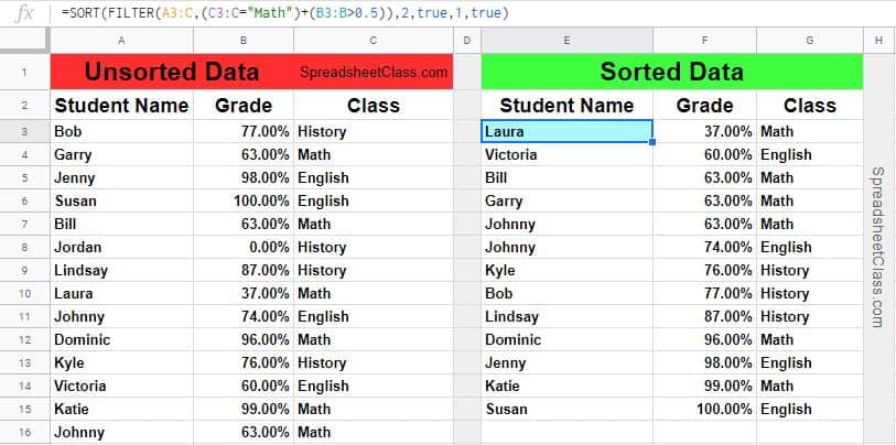
In this example we will also sort by multiple columns and filter by multiple conditions, but this time we will use “OR logic” for the filter criteria, meaning that either of the filter conditions cant be true to be included in the filter output. This is accomplished by separating the filter conditions with a plus sign, and wrapping the conditions in parenthesis.
The task: Filter the student data to show either math classes, or classes that are above 50%, and sort the result by grade and then by student name, both in ascending order
The logic: Filter the range A3:C, where C3:C is equal to the text “Math”, or where B3:B is greater than 0.5. Then sort the result by column 2 in ascending order, and then by column 1 in ascending order
The formula: The formula below, is entered in the blue cell (E3), for this example
=SORT(FILTER(A3:C,(C3:C=”Math”)+(B3:B>0.5)),2,true,1,true)

I hope that this helps you understand how to use the SORT and FILTER function together for your own task!
-Corey Bustos


