In this lesson I am going to teach you how to get a list of dates without weekends in your Google spreadsheet. I will also teach you how to use the WORKDAY function, which allows you to calculate a date that falls a certain number of workdays (business days) in the future or past, excluding weekends (and optionally, custom holidays). We will also go over the WEEKDAY function and how to use it as another method for getting dates without weekends.
First, let’s go over the basic use of the WORKDAY function, and then I’ll show you how to get a list of dates without weekends.
Get the future date after x many workdays with the WORKDAY function
Let’s say that you want to find out what the date will be after x many work days. This is exactly what the WORKDAY function does. First you specify the start date, and then you specify the numbers of workdays, and the WORKDAY function will provide you with the date that occurs after a specified number of workdays have elapsed from the initial start date.
To use the WORKDAY function in Google Sheets, follow these steps:
- Type =WORKDAY( to start the function
- Provide the cell reference or the date from which you want to begin counting workdays
- Type a comma
- Specify the number of workdays (positive for future dates or negative for past dates)
- Press the Enter key. The final formula will look like this: =WORKDAY(A2,B2) Where cell A2 contains the start date and cell B2 contains the number of workdays
After following the steps above, the selected cell will display the calculated date based on the specified start date and workday offset.
Example: Let’s say that we want to find what date will fall 10 workdays after the date 10/1/2023. To do this we will use the WORKDAY function as shown below (Where the start date is entered into cell A2 and the number of workdays is entered into cell B2).
=WORKDAY(A2,B2)

After following these steps, the cell will display the date 10/13/23, which is 10 workdays (business days) after the specified start date, excluding weekends.
The Google Sheets WORKDAY function description:
Syntax:
WORKDAY(start_date, num_days, [holidays])Formula summary: “Calculates the date after a number of working days from a specified start date.”
Get the past date before x many workdays with the WORKDAY function
If you want, you can use the WORKDAY function to provide you with the date that occurs a specified number of workdays before the initial start date.
=WORKDAY(A2,B2)

After following these steps, the cell will display the date 9/18/23, which is 10 workdays (business days) before the specified start date, excluding weekends.
Using the WORKDAY.INTL function to customize weekend days
If you want you can use the WORKDAY.INTL function to specify which days you want to be considered as weekends. This is done by a string of 1’s and 0’s, like this: “0000011” which indicates that Saturday and Sunday are weekend days and the rest of the days are not. The first number in the string represents Monday.
If you want Mondays and Tuesdays to be considered weekends, the string would look like this: “1100000”
=WORKDAY.INTL(A2,B2,”1100000″)

The formula above displays the date 10/15/23, which is 10 workdays (business days) after the specified start date, excluding custom weekends where Monday and Tuesday are considered weekends.
Get a list of dates without weekends with the WORKDAY function
Now that you know how to use the WORKDAY function, I will show you how to use it to generate a list of dates that exclude weekends.
To get a list of dates without weekends in Google Sheets, follow these steps:
- In another column, type =WORKDAY( to start the function
- Provide the cell reference or the date from which you want to begin counting workdays. Use the dollar sign to lock the row reference, like this: B$1
- Type a comma
- Use the ROW function as the reference for the number of workdays, like this: ROW(A1)
- Press the Enter key. The final formula will look like this: =WORKDAY(B$1,ROW(A1))
- Copy the formula down the column.
Method 1: Using a numbered list and the WORKDAY function
Let’s go over the method that is most intuitive, and then we will go over the ROW function method which makes more sense after you learn the method using a numbered list.
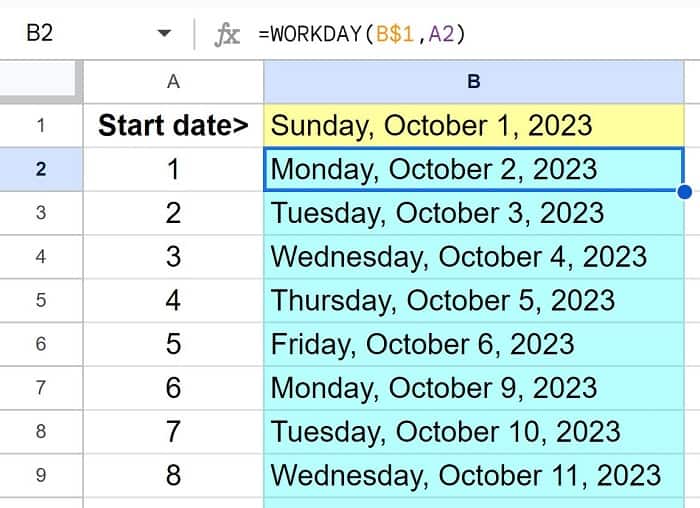
First we will use column A to create a list of numbers, where the numbers increments 1 for each row. To do this simply enter the number 1 into cell A2, enter the number 2 into cell A3, then highlight cells A2 and A3, then use the fill handle to quickly make a sequence of numbers in column A.
Then we will refer to this incrementing list of numbers with the WORKDAY function, so that the function generates a list of dates without weekends as the WORKDAY function is copied down the column.
=WORKDAY(B$1,A2)

As you can see in the image above, we have created a list of dates that contain only workdays, and do not contain dates on weekends. If you want you can copy and paste these dates as values only somewhere else in your spreadsheet, so that you have the list of dates without the formulas.
Method 2: Using the ROW function with the WORKDAY function
If you prefer, when you are generating a list of dates without weekends, you can use the ROW function with the WORKDAY function, instead of entering a sequence of numbers into a column.
The formula below will achieve the same result as the formula in the example above. You may find this method easier since you don’t need to create a numbered list. But I find that understanding the numbered list method helps to better understand how this ROW function method works.
=WORKDAY(B$1,row(A1))
Copy dates as values only
To do this copy the cells that contain the dates that you want to copy by pressing Ctrl +C on the keyboard, and then after you select the cell where you want to paste press Ctrl + Shift + V on the keyboard to paste values only.
In this example the dates were formatted to display the day of the week so that you can easily see how the weekend days are being skipped in the date sequence.
Customize weekends in your list with the WORKDAY.INTL function
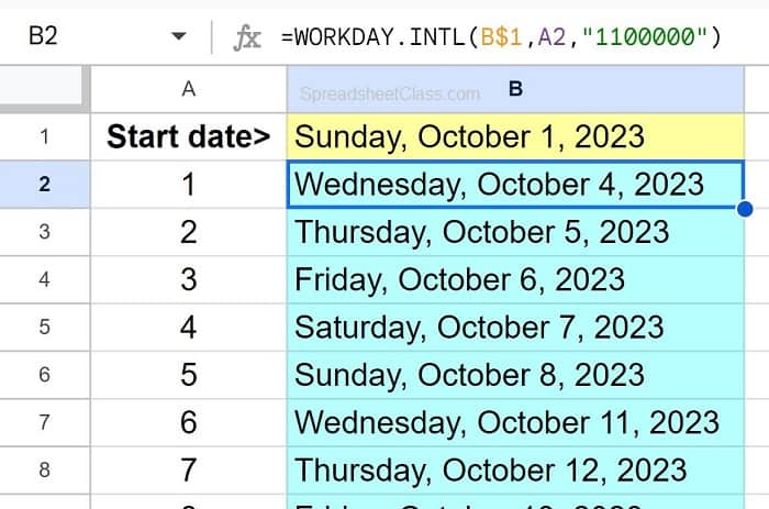
The WORKDAY.INTL function can also be used to generate a list of dates without weekends, where the days that represent weekends are customized by you. Just like how we used this function in a previous example, the weekends days are specified by a string of 7 1’s and 0’s, like this: “1100000” which represents that Monday and Tuesday should be counted as weekend days (and that all other days are considered as workdays).
The example below is the same as the previous example, except that weekends have been customized. Notice how the list of dates generated now skip Monday and Tuesday dates.
=WORKDAY.INTL(B$1,A2,”1100000″)

Using WEEKDAY and FILTER to create a list of dates without weekends
Now I’ll show you my preferred method of creating a list of dates without weekends. Even though this method uses two different formulas, I find this method easier to understand.
You can utilize the WEEKDAY function in combination with the FILTER function to create a custom list of dates without weekends, where the WEEKDAY function shows the day of the week for each date in a sequence of dates, and the FILTER function filters the data to only display the days of the week that you choose.
The get a list of dates without weekends with the WEEKDAY and FILTER function, follow the steps below:
Step 1: Use the WEEKDAY Function to display the day of the week
Enter a sequence of dates in column A.
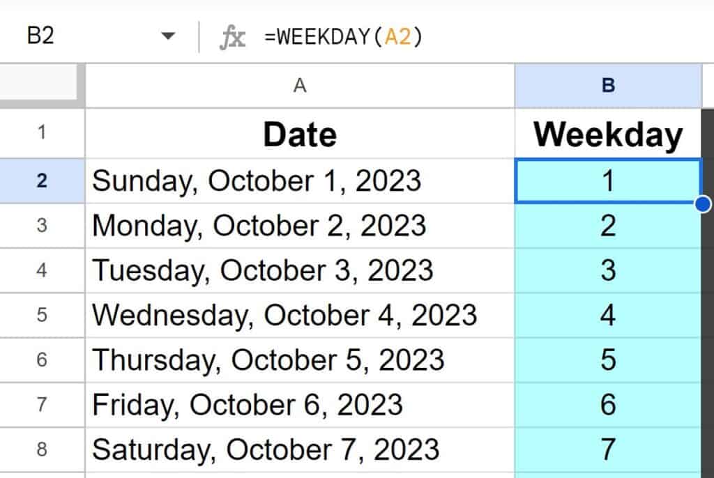
Then use the WEEKDAY function in column B to determine the day of the week for each date in the list / column. The WEEKDAY function returns a number representing the day of the week, with Sunday being 1, Monday being 2, and so on.
Enter the following formula in cell B2 to calculate the day of the week for the date in cell A2, and then copy the formula down the column to do the same for each date:
=WEEKDAY(A2)

As you can see in the image above, column B now shows a number in each row that represents the day of the week for each date. This will allow us to use the FILTER function to exclude or include whichever days that we want in the filter results.
The Google Sheets WEEKDAY function description:
Syntax:
WEEKDAY(date, [type])Formula summary: “Returns a number representing the day of the week of the date provided.”
Step 2: Create a Filtered List
Now, you can use the FILTER function to create a filtered list of dates based on the WEEKDAY results. The FILTER function allows you to select rows from a range that meet specific criteria.
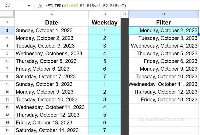
In an empty cell, let’s say cell D2, enter the following formula to create a list of dates without weekends:
=FILTER(A2:A15,B2:B15<>1,B2:B15<>7)

This formula tells Google Sheets to filter the dates in cells A2 to A15, excluding any rows where the corresponding day of the week (from the WEEKDAY function in column B) is either 1 (Sunday) or 7 (Saturday). Adjust the range (A2:A15) as needed to match your data.
In this example we used the not equal sign to show filtered results that do not meet a specified criteria. If you want you can also use the filter function to specify criteria that you do want to be contained in the results, such as specifying the days that you do want to include, rather than excluding the days you don’t want to include. You can learn more about using the FILTER function here.
Now you know how to get dates without weekends in Google Sheets!

