Many people don’t know that you can hide the toolbar menu in Google Sheets, but in this lesson I will show you 2 super easy ways to hide the menu in your Google spreadsheet. This will make the view of the spreadsheet cells larger, and cleaner.
This is really handy for when you have a presentation to share, a dashboard, or if you simply want to view more cells on your sheet, especially when you have a small computer screen.
There is a button that will allow you to hide the menu, and a keyboard shortcut. In this article I will teach you both ways.
How to hide the toolbar menu with a button
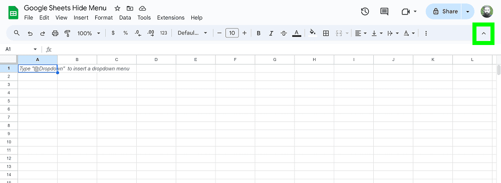
To hide the toolbar menu in Google Sheets, click the button on the upper-right of the screen that looks like a caret or a triangle pointing upwards. This button is directly below your Google profile picture.
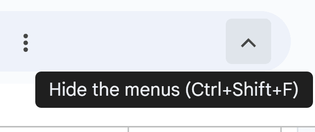
The image below shows the “hide the menus” button, and as you can see when you hover your cursor over the button it will display the keyboard shortcut, which we will go over later.

Below you can see what the Google spreadsheet looks like by default, with the top toolbar menu displayed. The button to hide the menu is highlighted in green.

Click the “hide the menus” button, and the top menu will be hidden, as shown in the image below.
After doing this the top menu will take up less room, and there will be more room to display the spreadsheet cells.

Hide the menu with a shortcut
You can also use a keyboard shortcut to hide the menu in Google Sheets.
To hide the menu with a shortcut in a Google spreadsheet, simply press Ctrl + Shift + F on the keyboard.
Keyboard shortcut to hide menu in Google Sheets:
Ctrl + Shift + F
Show the menus
Showing the menus when they are hidden, is the same exact process as hiding the menus. Simply choose one of the methods above, either click the button or use the keyboard shortcut to show the toolbar menu.

